Normal view

There are new articles available, click to refresh the page.
Before yesterdayMain stream

Reveal SAP EWM – Warehouse Order sorting in Queues

Reveal SAP EWM

Sorting of Warehouse orders within Queues

My new blog post is offers a comprehensive summary of warehouse order sorting in queues. I delve deep behind the scenes and reveal a few secrets along the way.

The article begins with the basics, explains sorting with and without pre-assignment of warehouse orders to resources, and concludes with an analysis of the logic in the context of physical inventory and task interleaving.

Context

It is important to understand that we are only talking about the sorting within one queue. With a system-guided selection or with a task interleaving approach the resource group of the current resource might be assigned to multiple queues and the queue sequence as such is evaluated before the sorting within one queue becomes relevant. With this article however, we are looking at one single queue only and the sorting within this queue. 

Also certain warehouse orders in the queues might not be considered for the resource type of the resource which the current user used to login (e.g. resource execution constraints). This filtering of warehouse orders is also not in scope for this article as it has no impact on the actual sorting of applicable WOs. To say it again – Pure sorting, nothing else!

Agenda for this blog-post

  • Main part: How are WOs technically being sorted in a queue?
    • How does the EWM standard sort the WOs within the queues? Which factors have an impact? How are those factors being calculated?
    • How does this sorting logic change in case multiple WOs are pre-assigned to the current resource?
    • What options does EWM offer to implement a custom logic for the sorting?
  • Party-knowledge
    • Sorting of WOs for physical inventory
    • Sorting while interleaving being active

How does the sorting work?
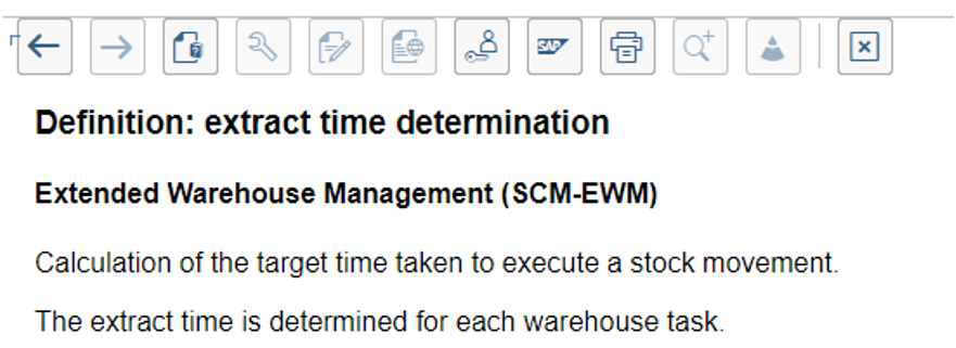
Let us start again from the SAP help text

If more than one WO falls within any of these queue classifications, the WOs are sorted as follows:
In ascending order, by latest starting date (LSD)
In descending order, by execution priority.

So we learned that the sorting depends on two values:

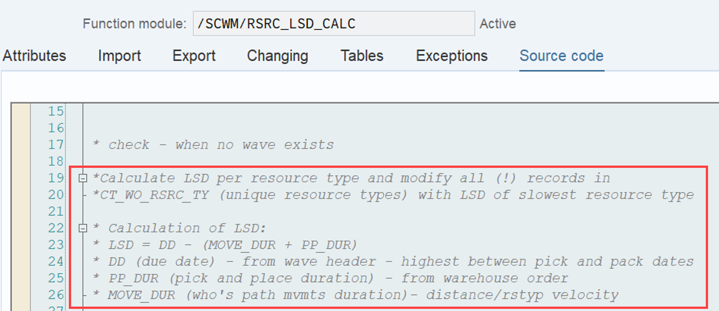
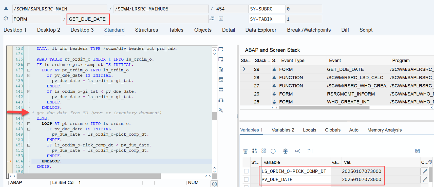
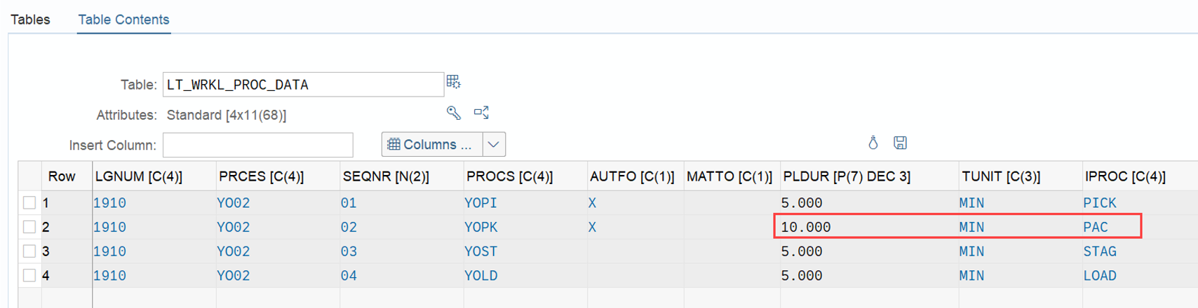
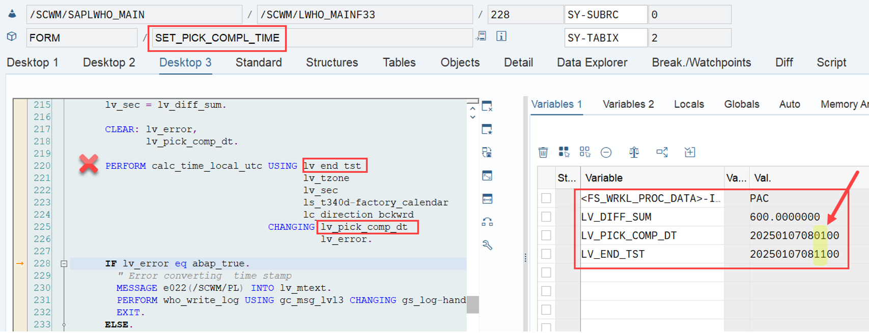
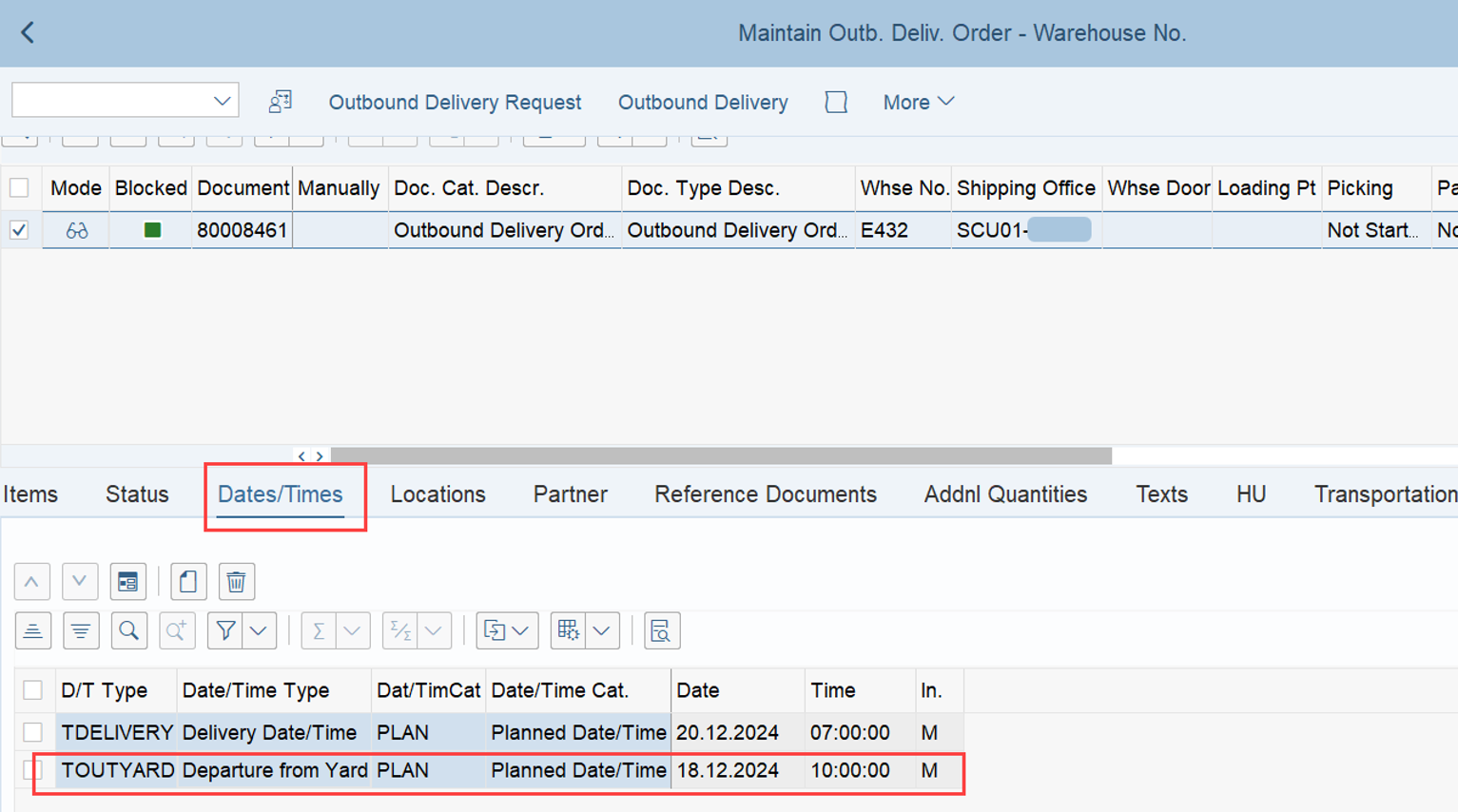
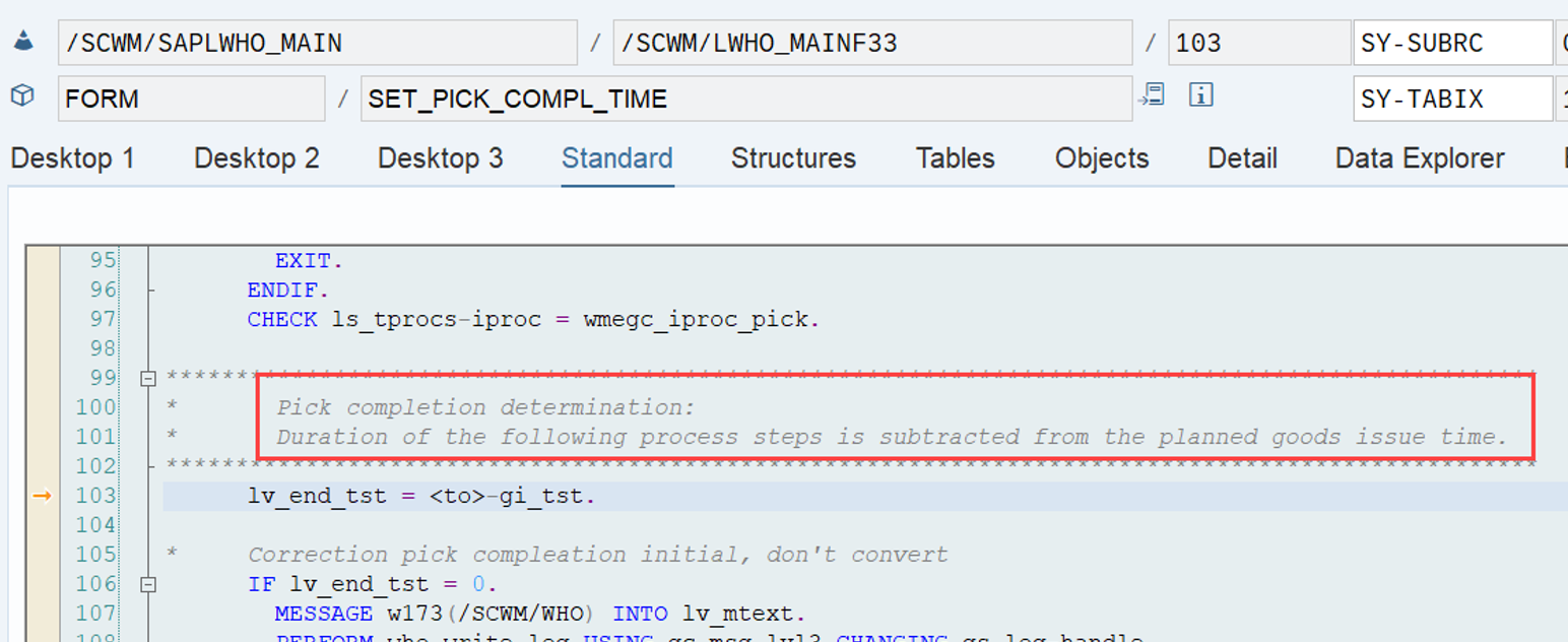
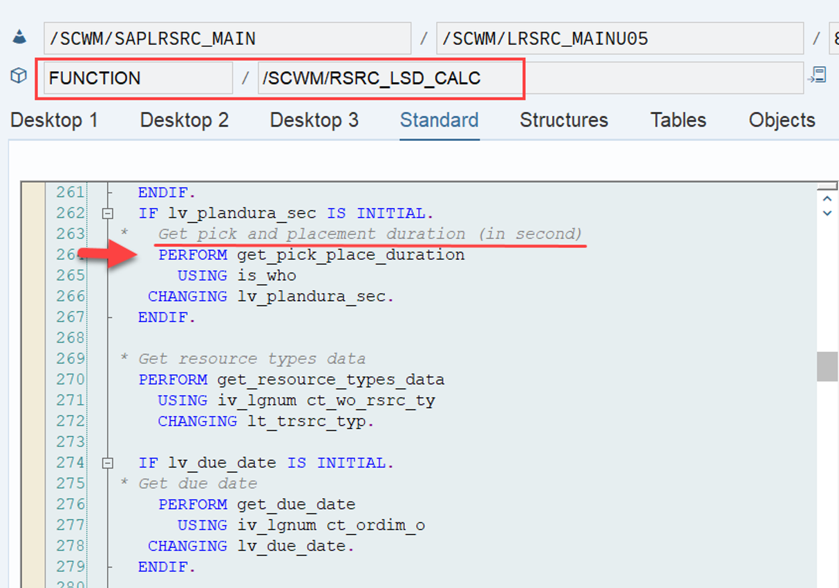
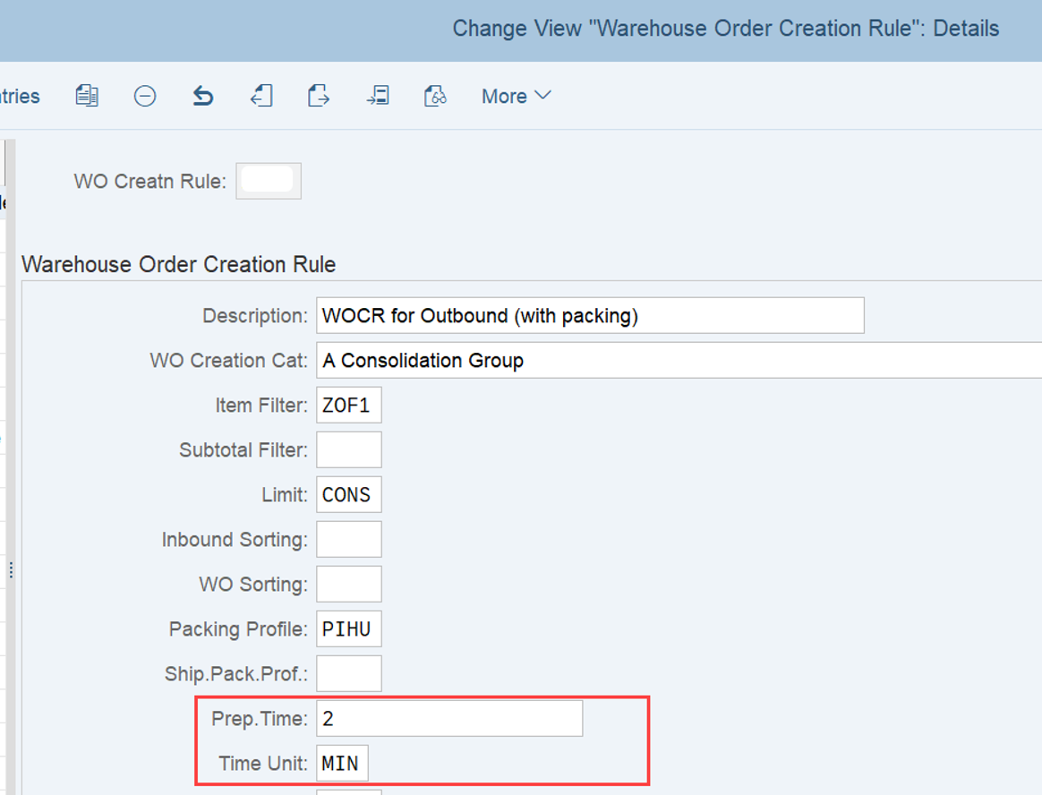
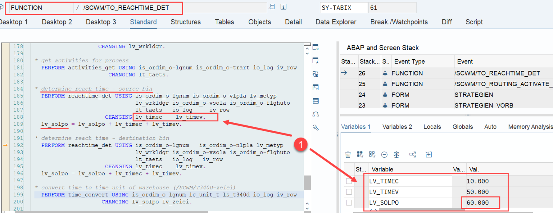
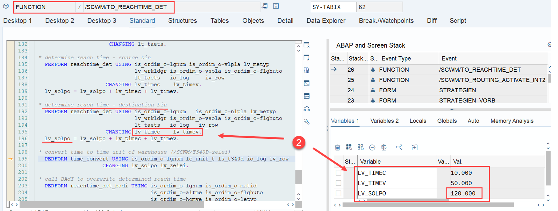
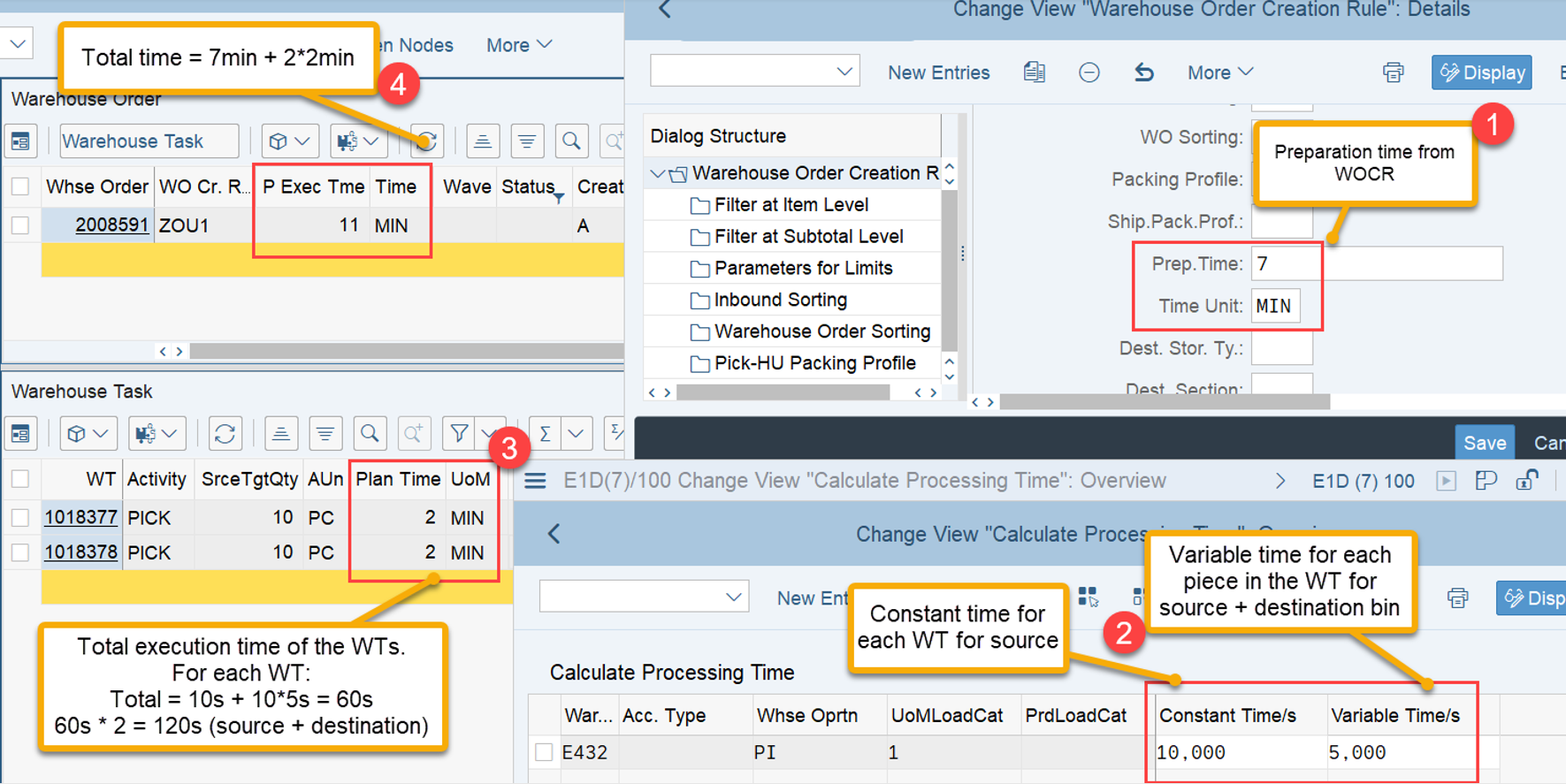
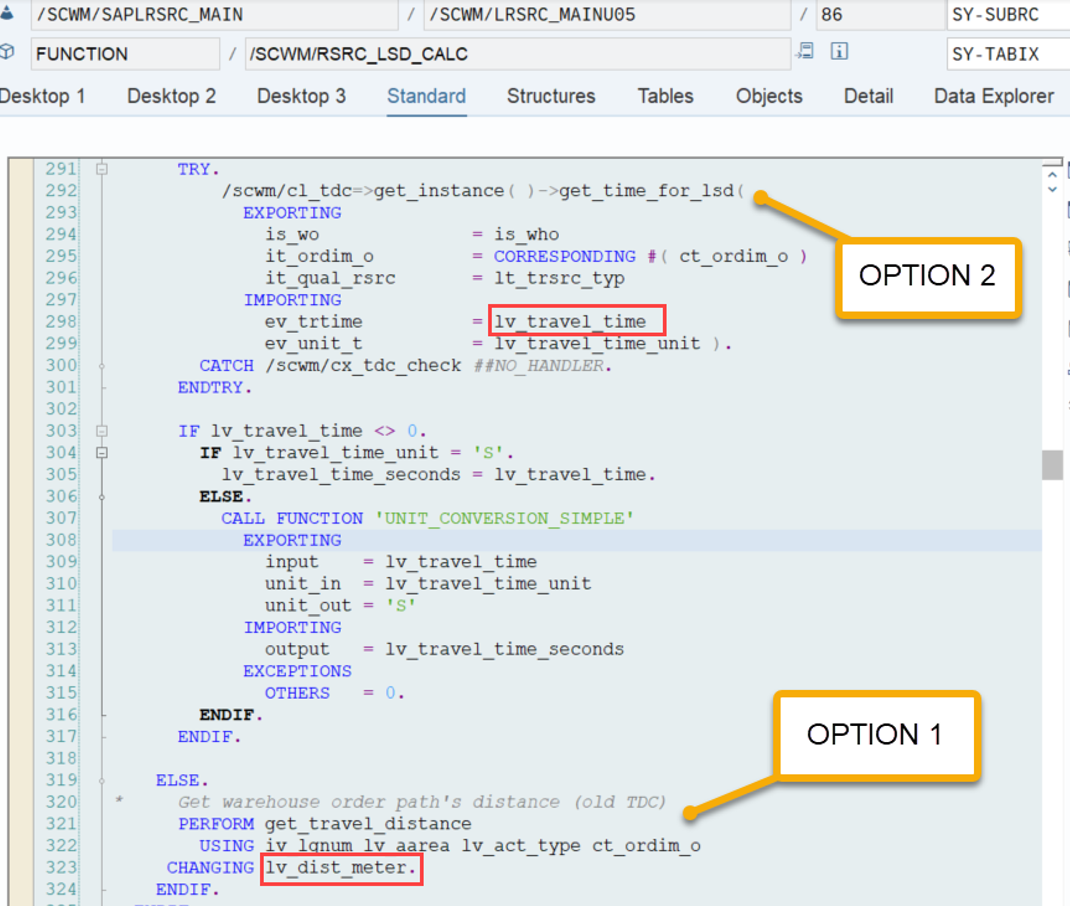
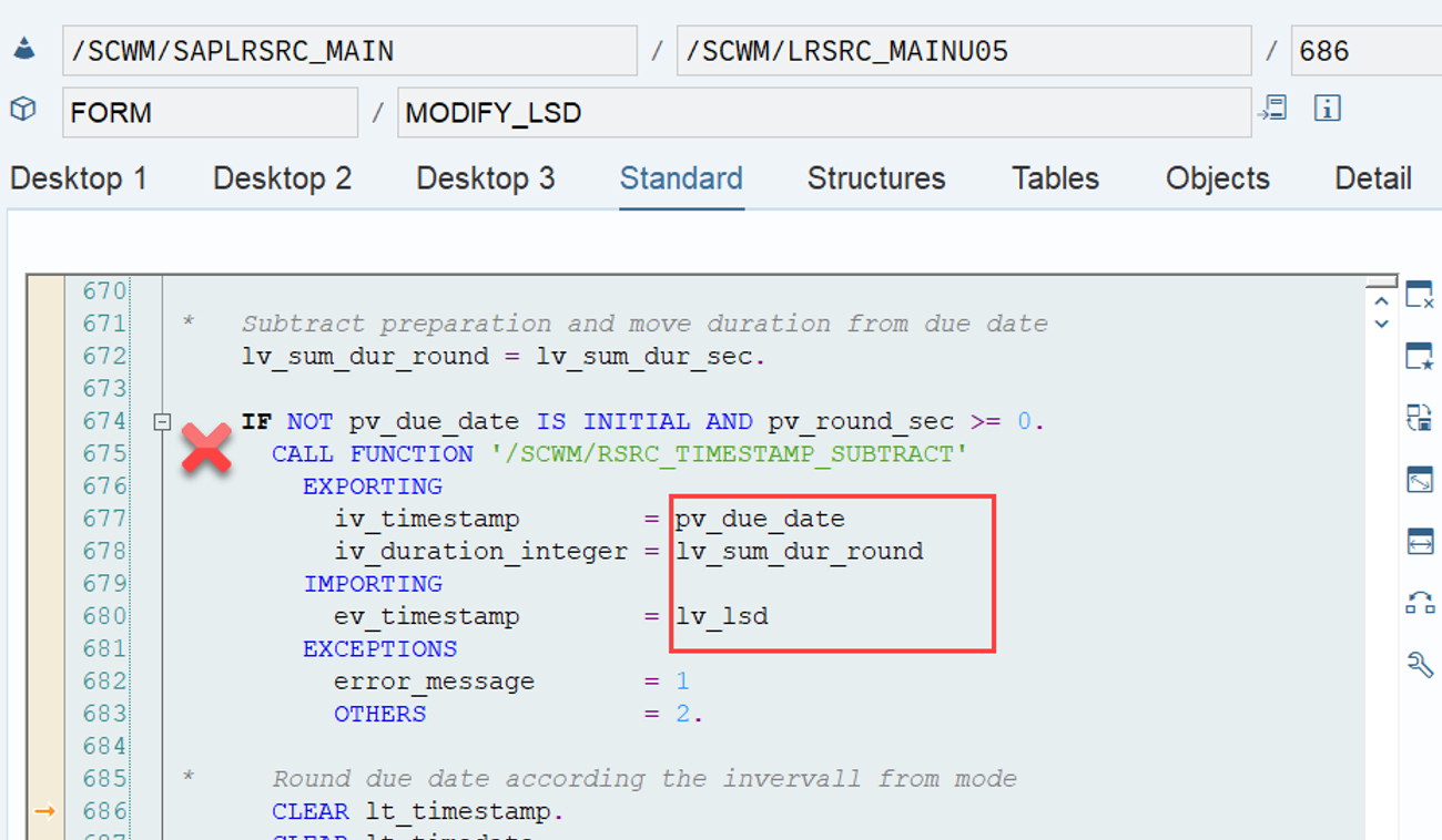
LSD calculation: This is explained in my other video or blog-postIt is calculated based on the following formula: LSD = WO due date – (planned execution duration + planned movements duration)

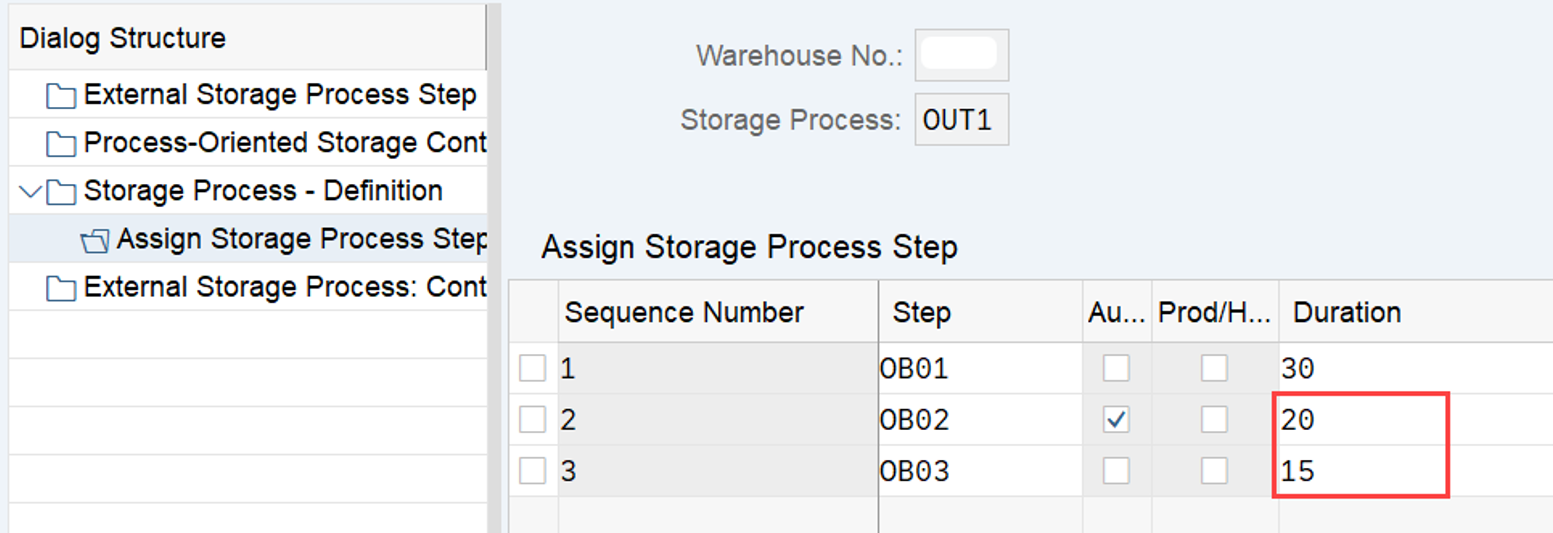
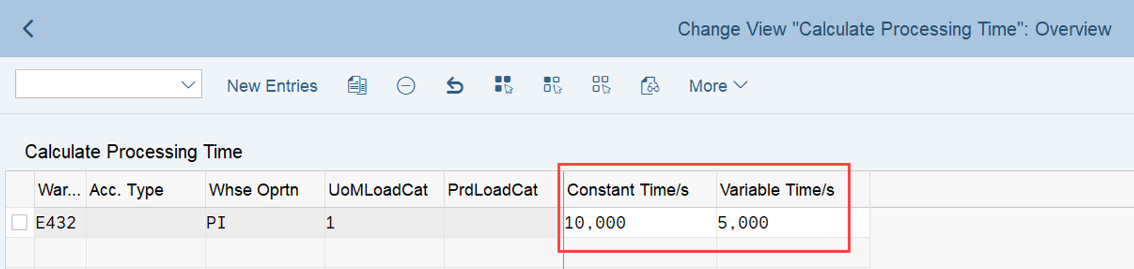
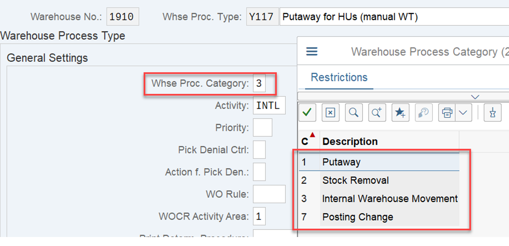
WO Prioritization: This has a good SAP help text with lots of examples for the calculation. For each WT in the WO the priority is calculated with the following formula: Priority = (BAT Weighting/100 x BAT Priority Value) + (HUTG Weighting/100 x HUTG Priority Value) + (WPC Weighting/100 x WPC Priority Value). The WO priority is then set to the priority of its WT with the highest priority value.

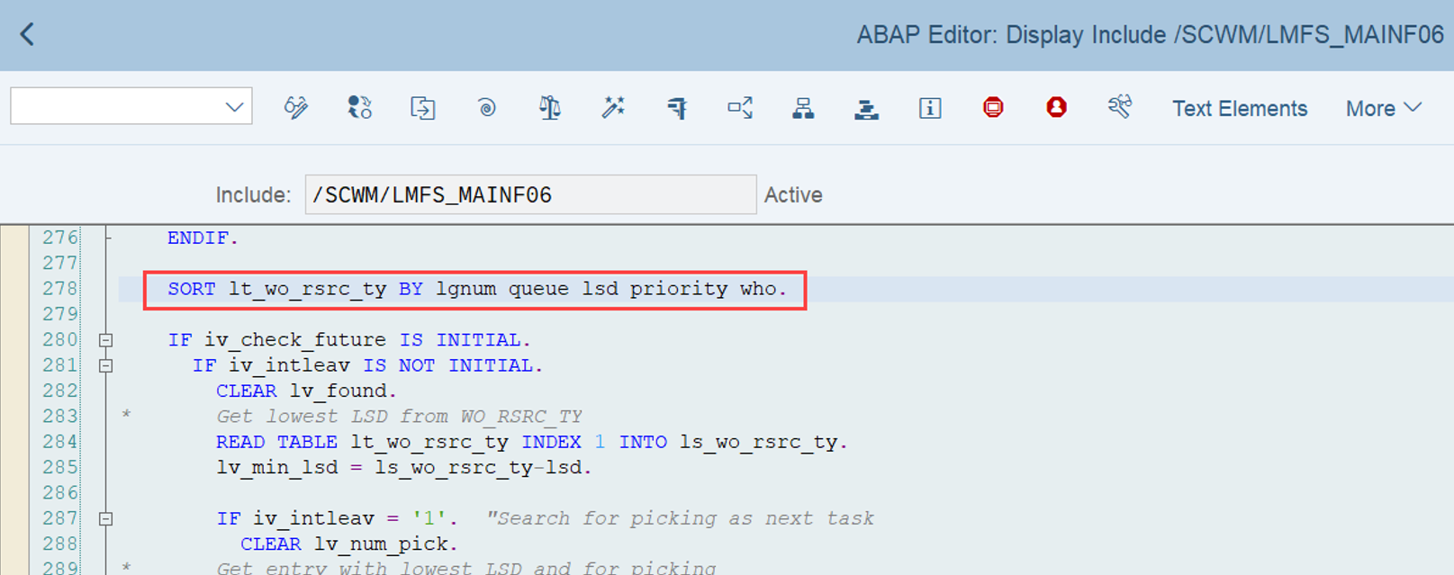
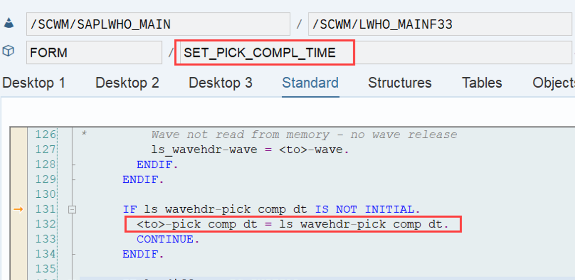
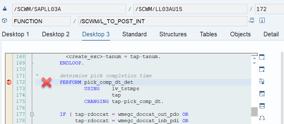
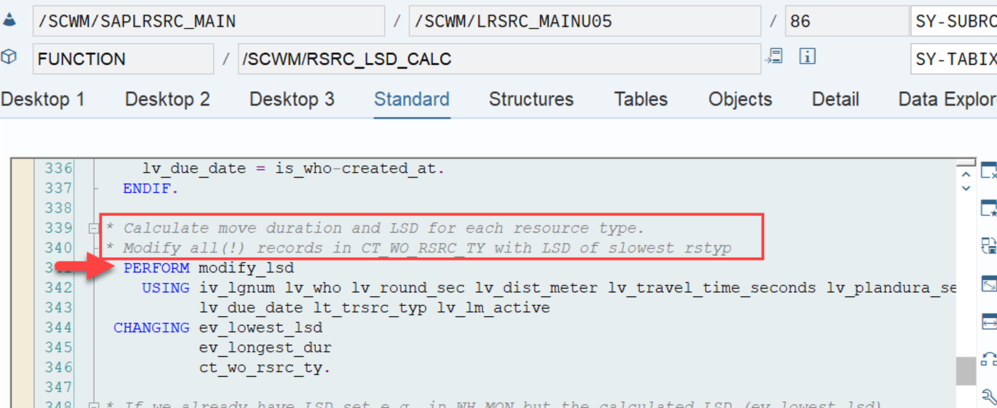
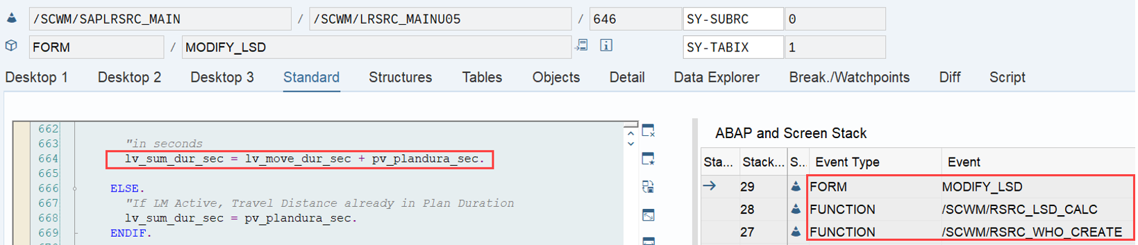
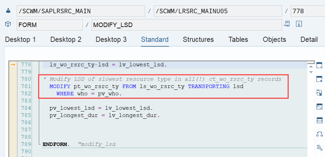
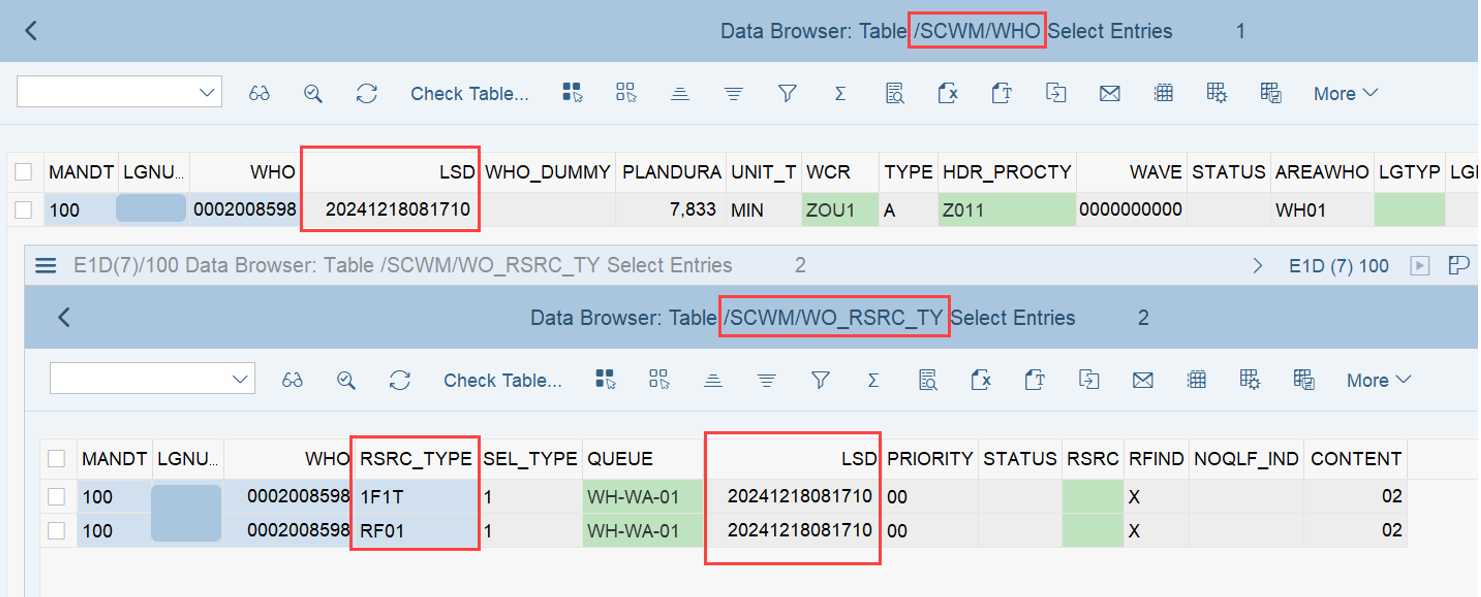
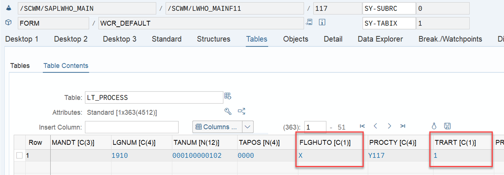
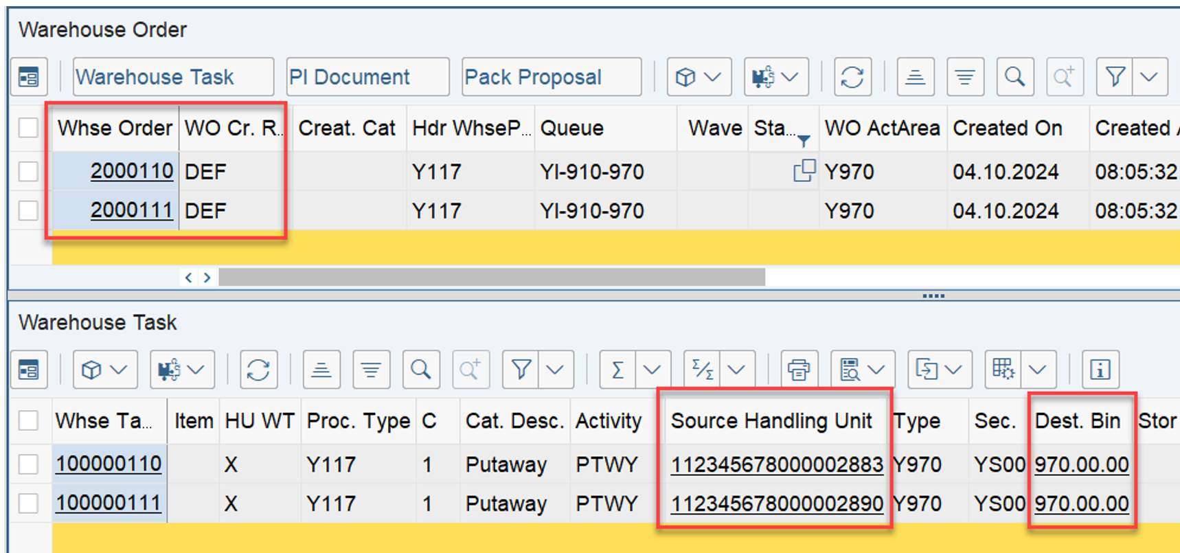
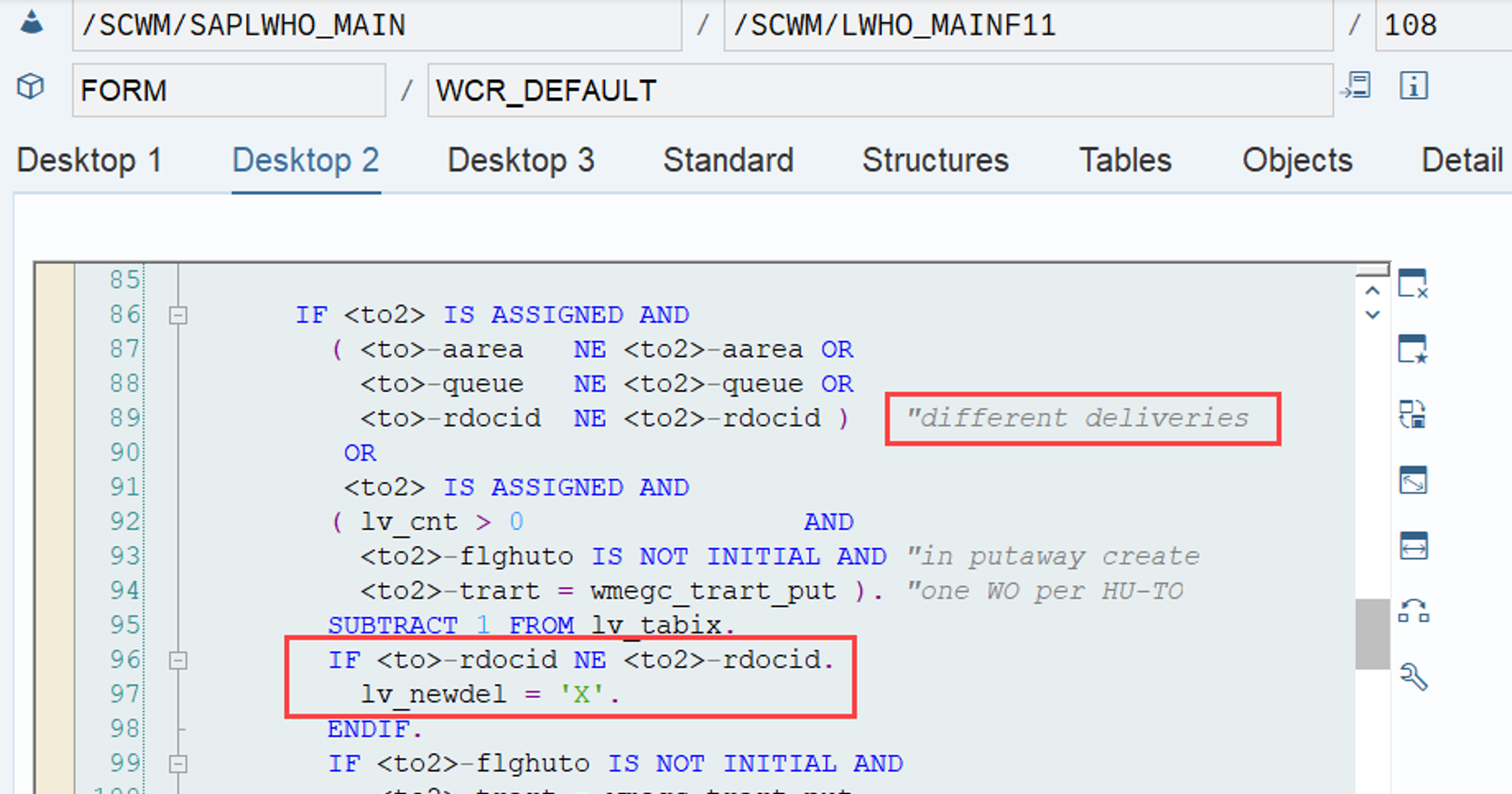
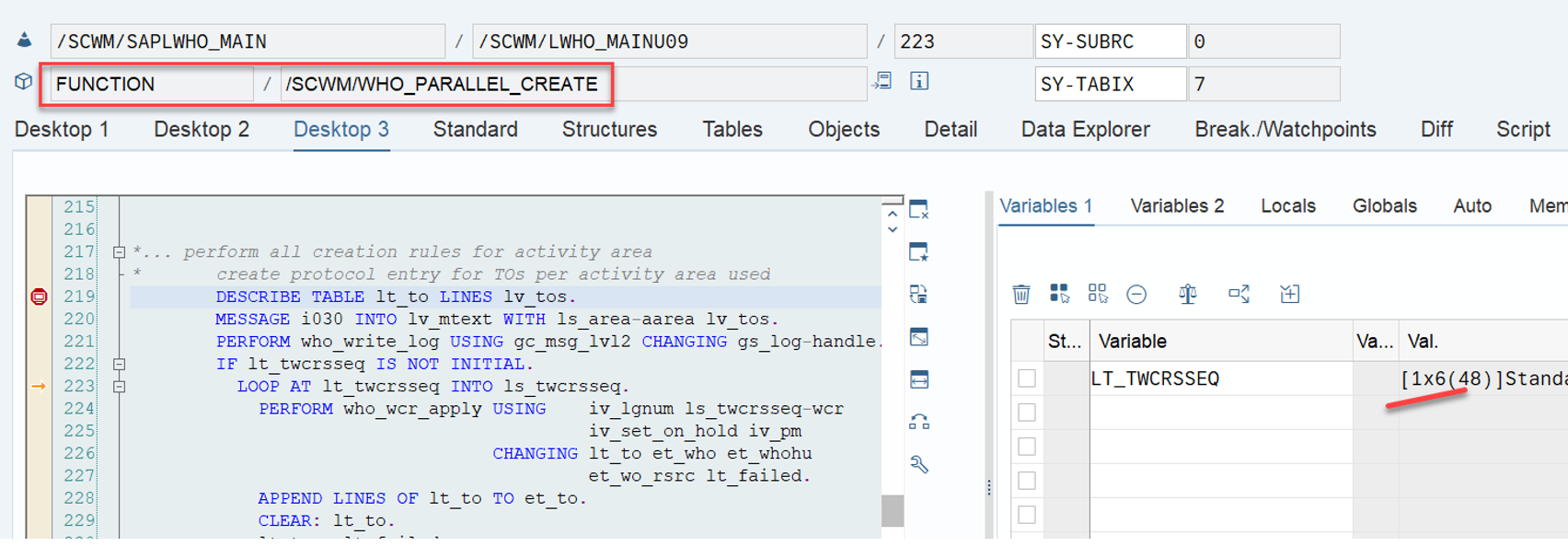
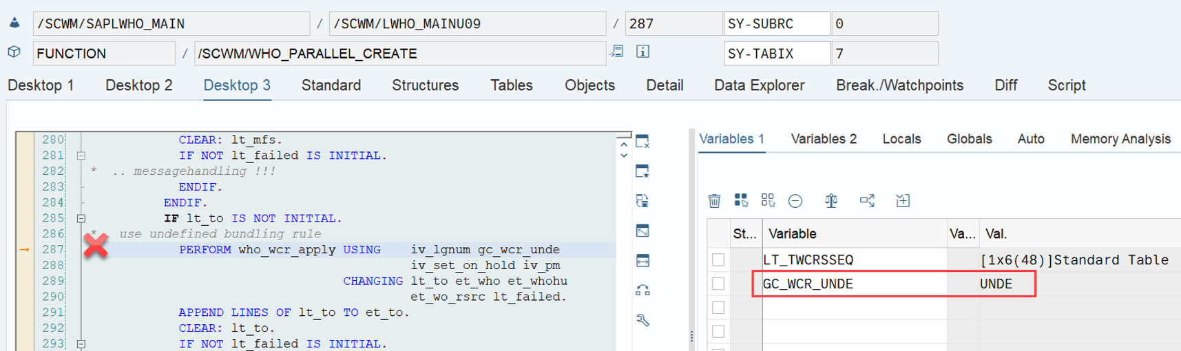
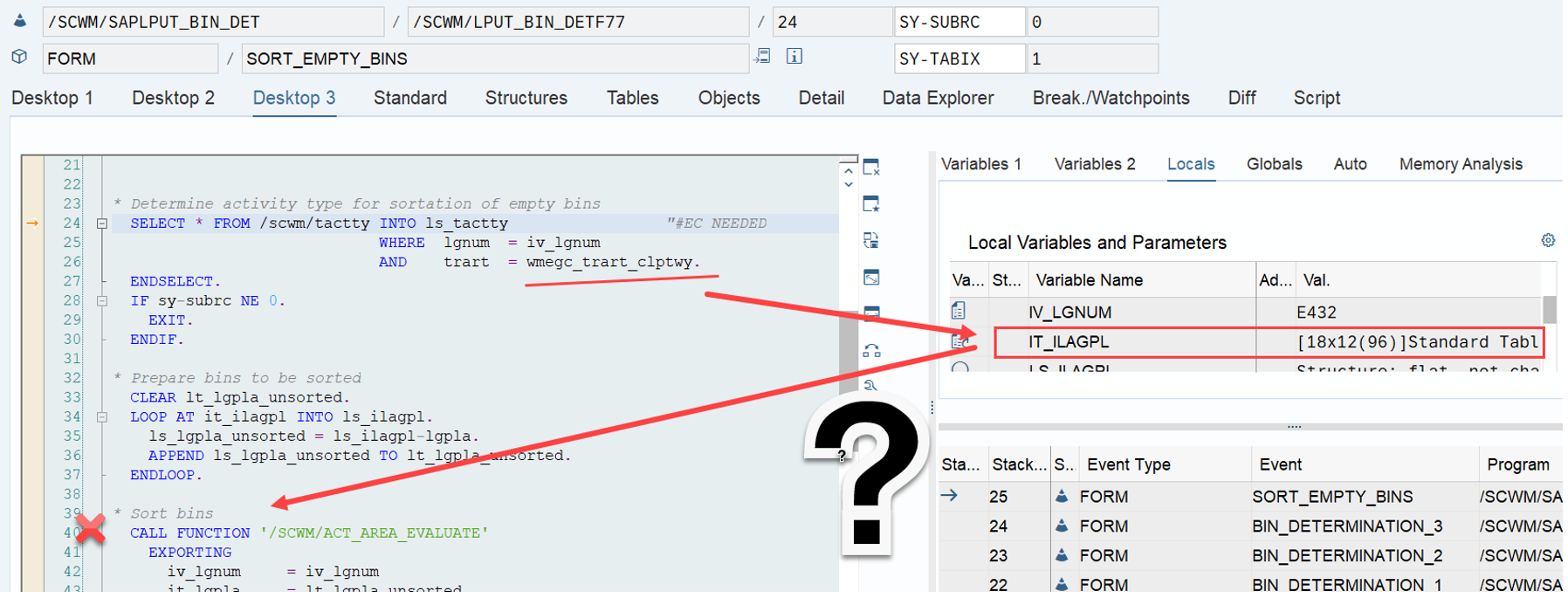
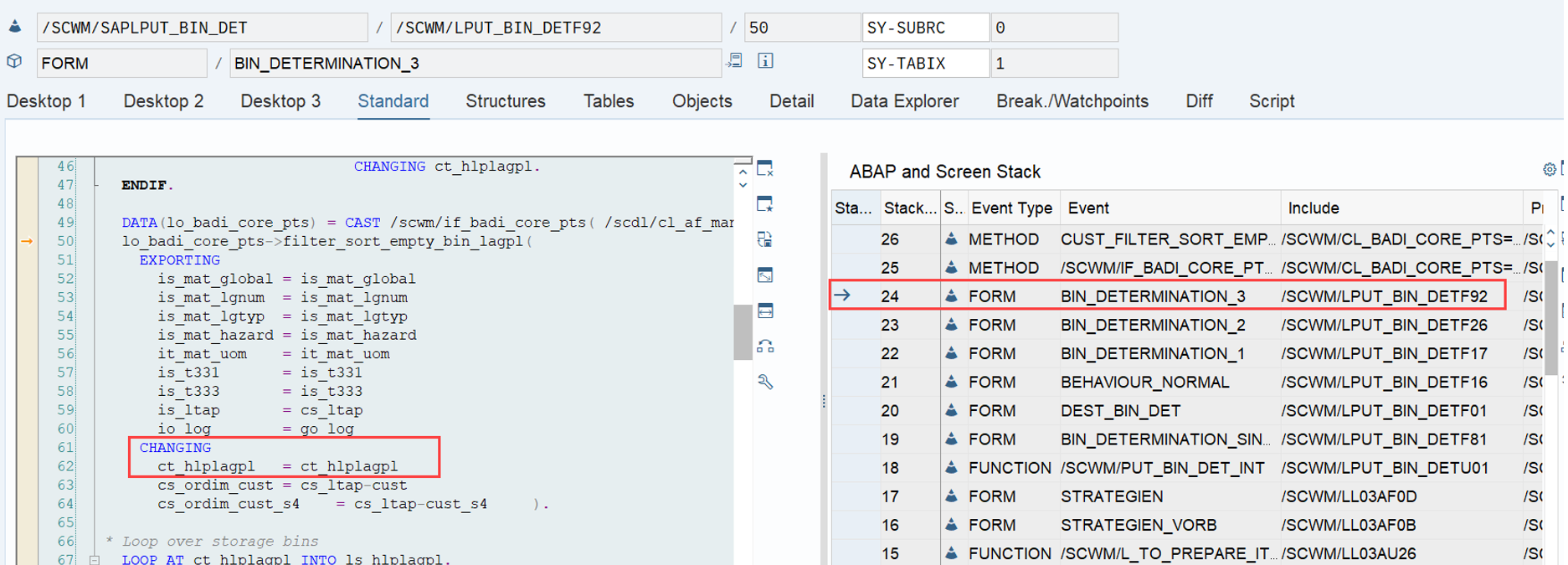
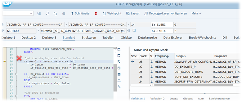
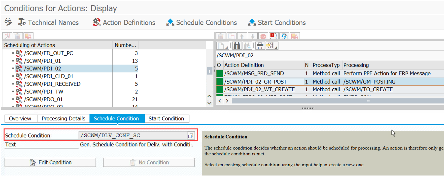
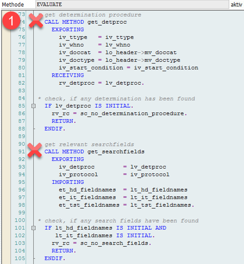
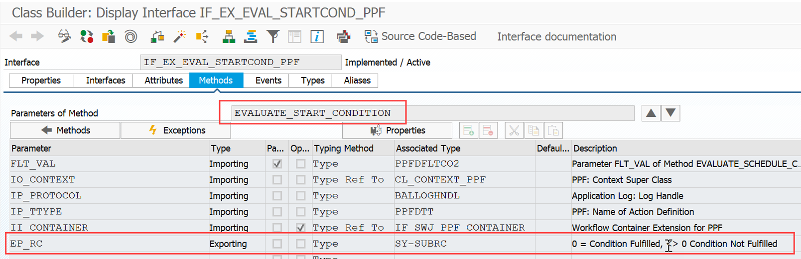
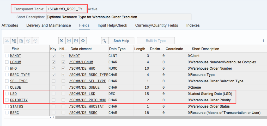
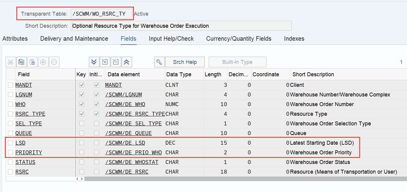
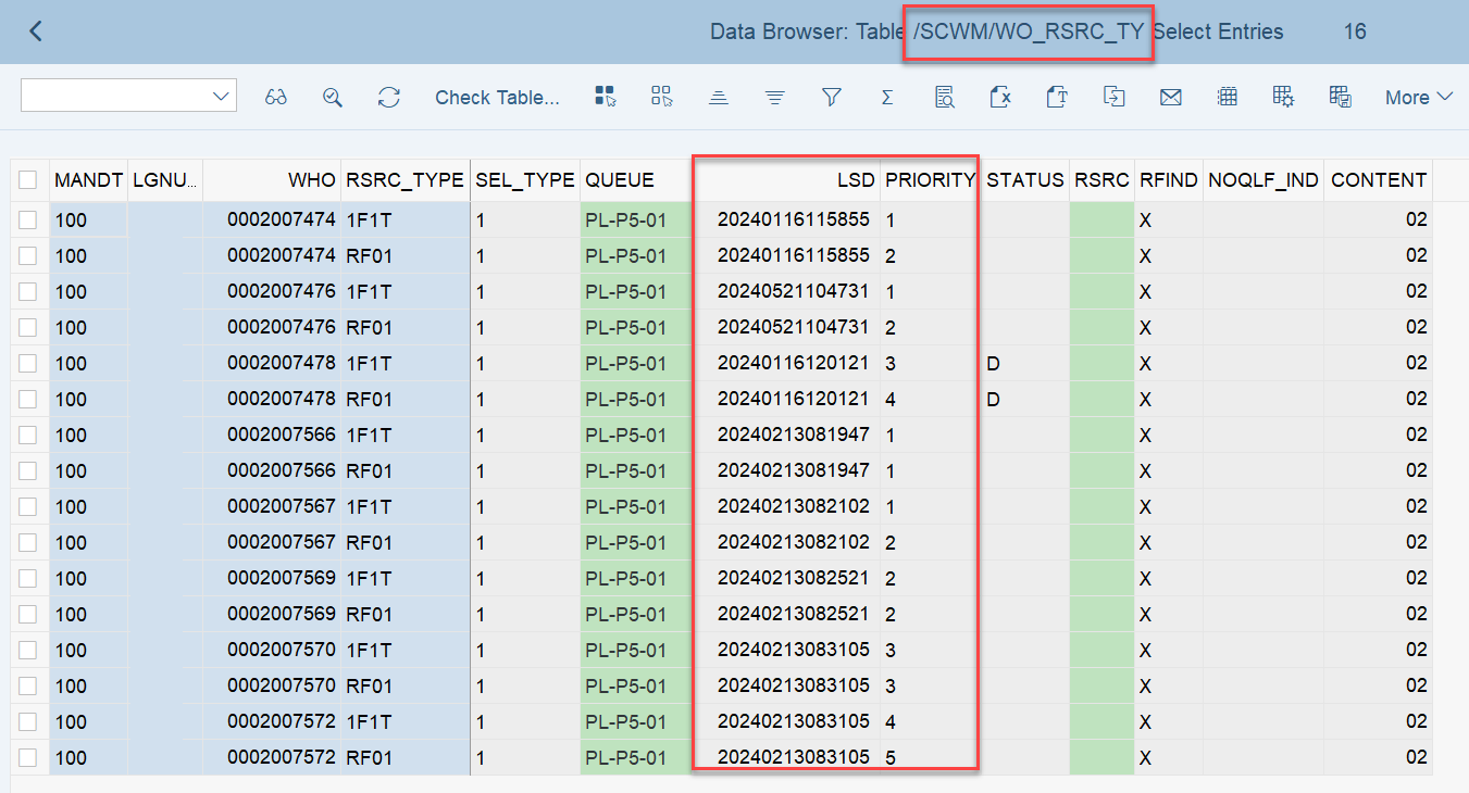
Important: Both values are calculated during warehouse order creation, well before the actual sorting occurs during warehouse order processing. Therefore, if you change your customization settings later, do not be surprised if nothing changes. Both values are saved in the table /SCWM/WO_RSRC_TY (the LSD is also saved in table /SCWM/WHO, but this table is not relevant for our context here). The calculation for both values is initiated by the function module FM /SCWM/RSRC_WHO_CREATE during warehouse order creation, which also calls FM /SCWM/WHO_RSRC_TYP_SET to write the result to the database.

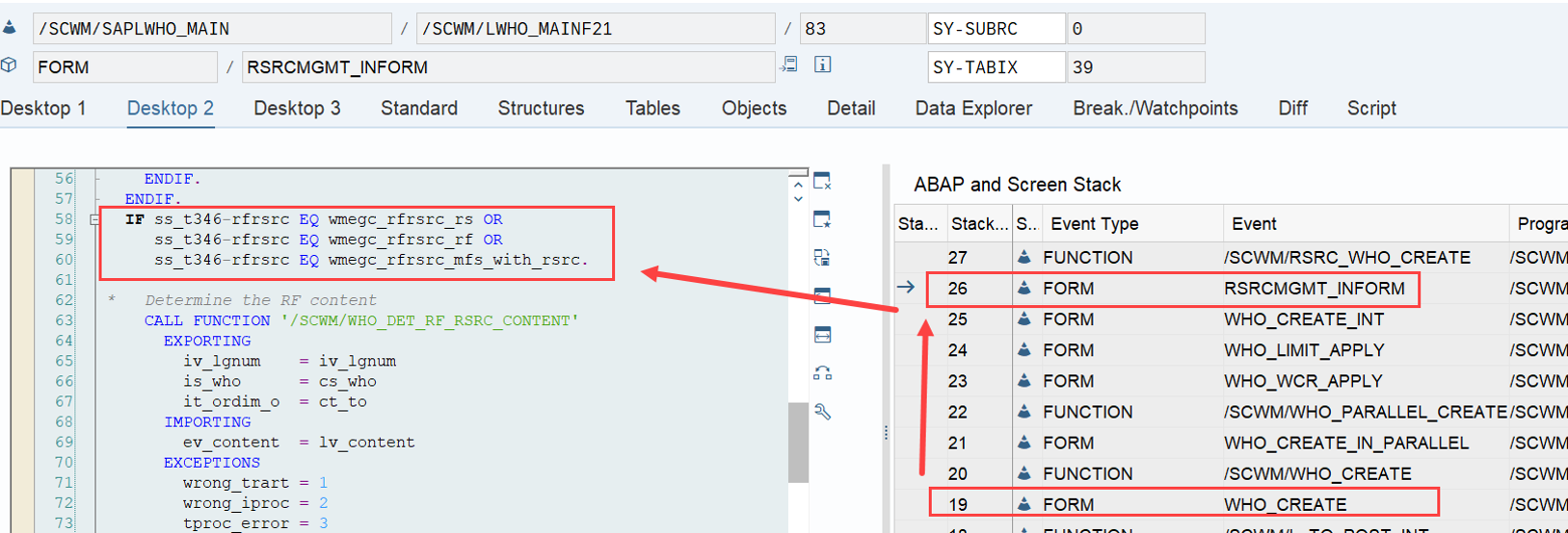
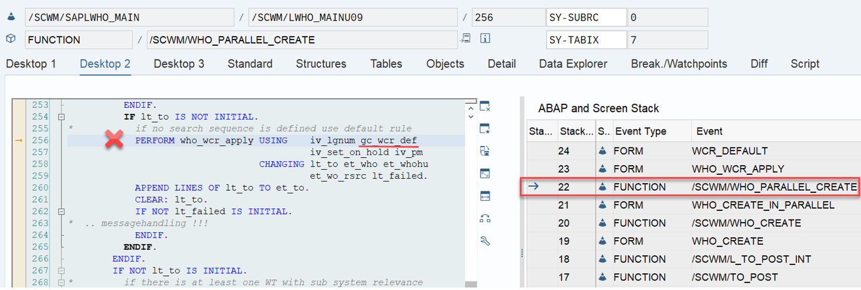
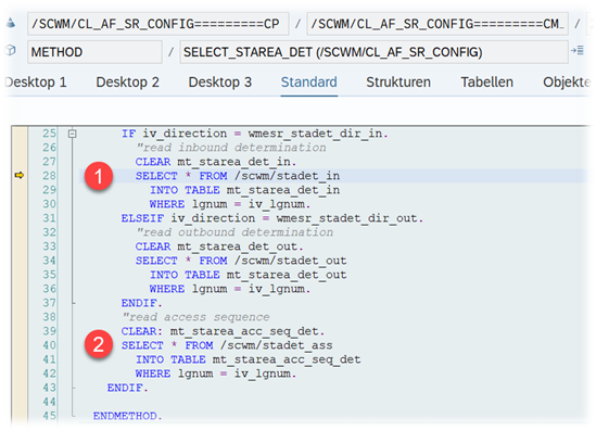
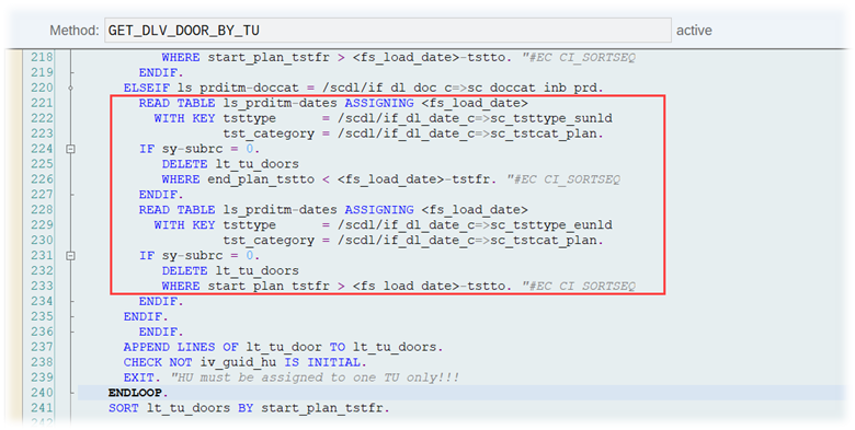
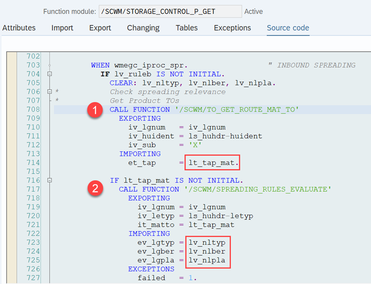
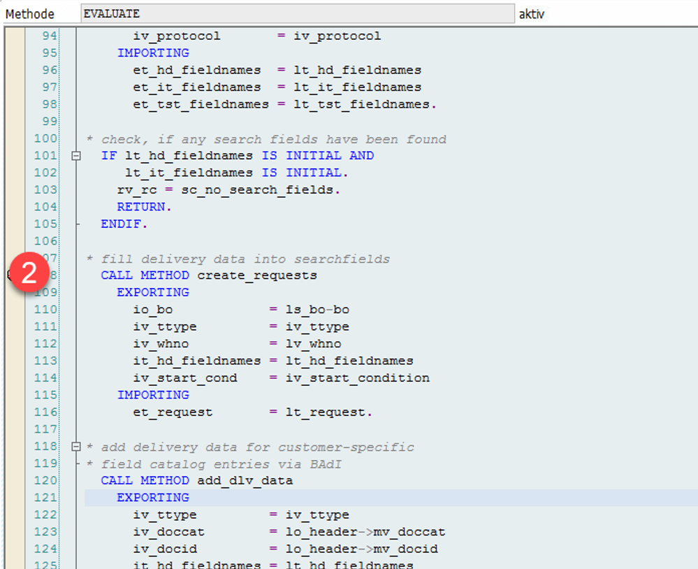
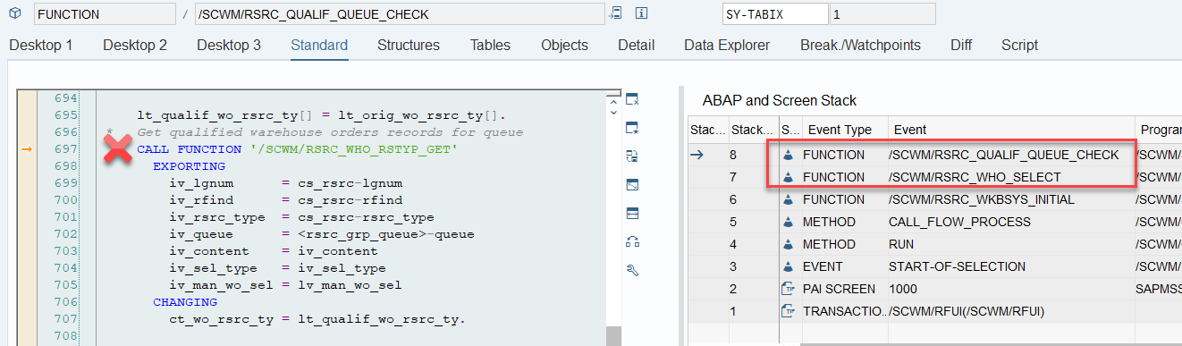
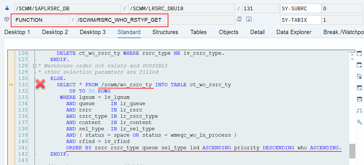
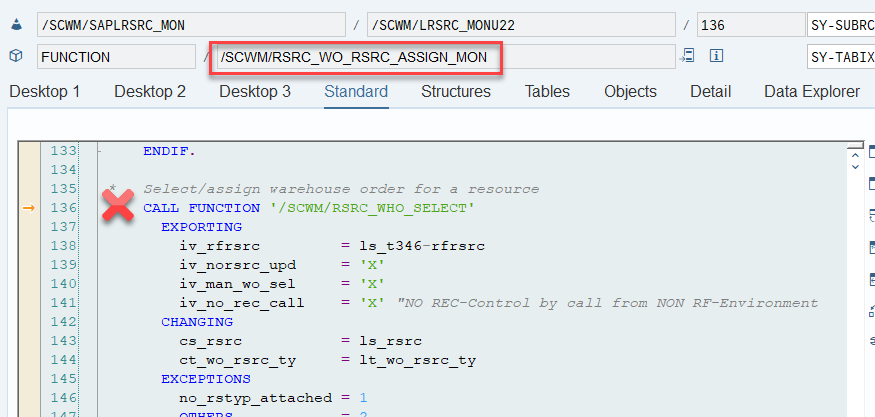
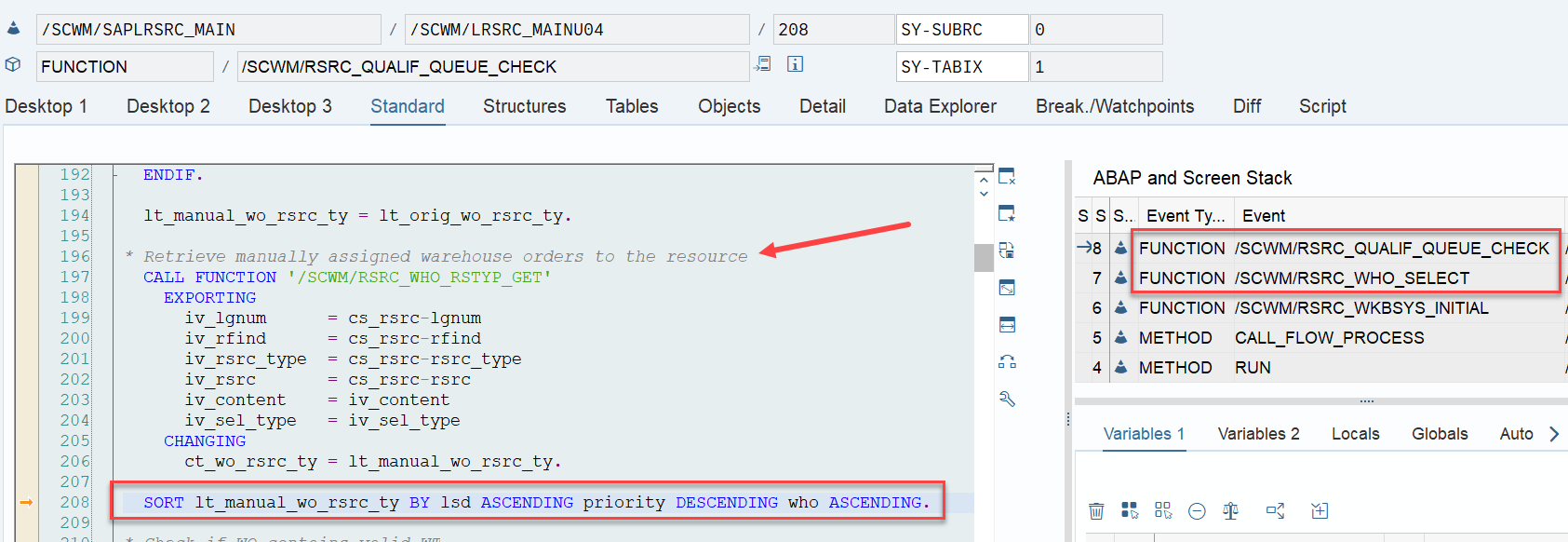
During warehouse order processing, EWM selects records from this table and sorts them accordingly. This process is executed via the function module /SCWM/RSRC_WHO_SELECT, which calls FM /SCWM/RSRC_QUALIF_QUEUE_CHECK, and subsequently calls FM /SCWM/RSRC_WHO_RSTYP_GET. This FM reads the table entries from /SCWM/WO_RSRC_TY before filtering and determining the applicable warehouse orders for the given resource type (details of which are not explained here)

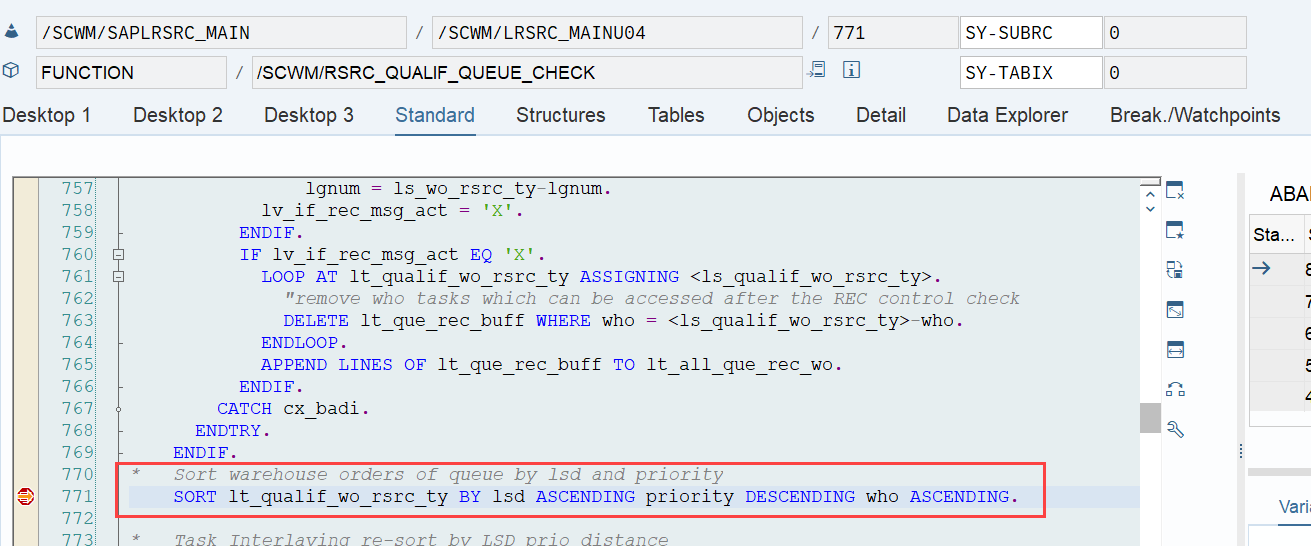
The same sorting is applied again a few lines later when the internal table is handed over to the calling function module FM /SCWM/RSRC_QUALIF_QUEUE_CHECK. This seems redundant, but there could be technical reasons for it (Is a developer amongst you able to explain the technical reason for sorting two times here in the comments of the corresponding video!?).

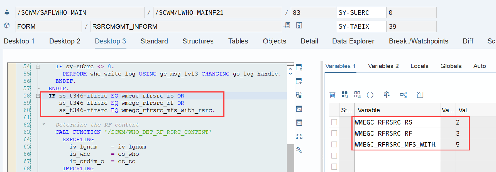
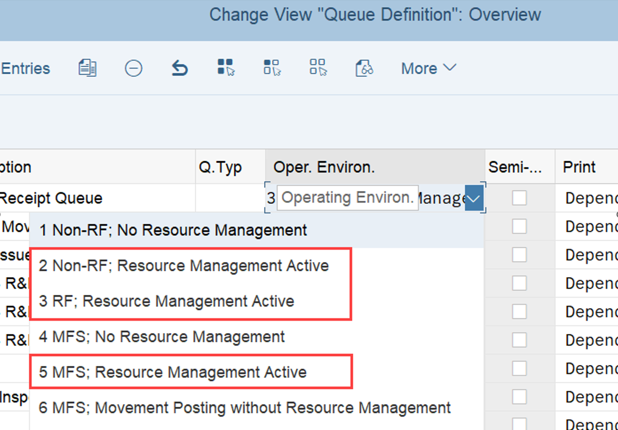
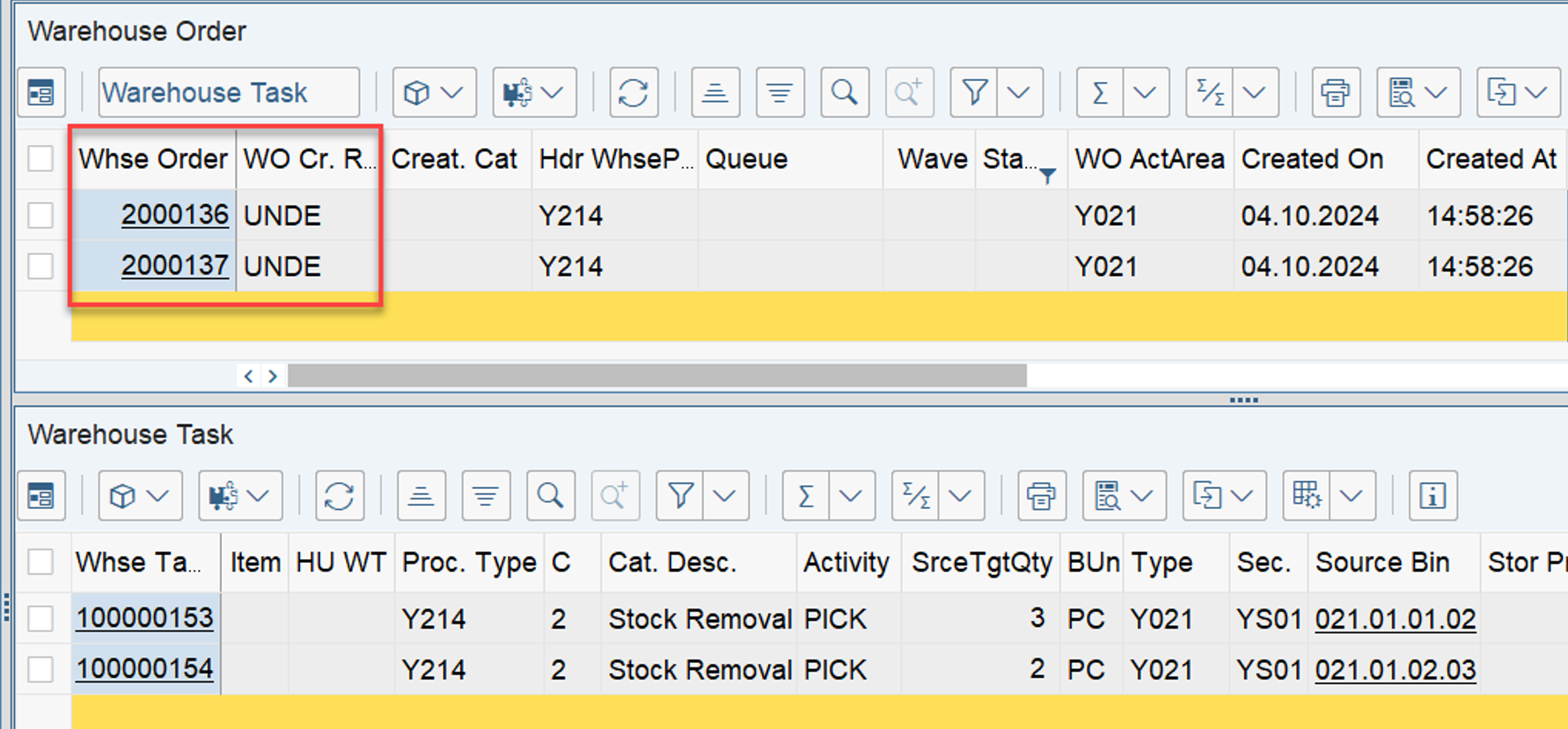
The example below highlights the way of sorting, based on the 3 values listed above:

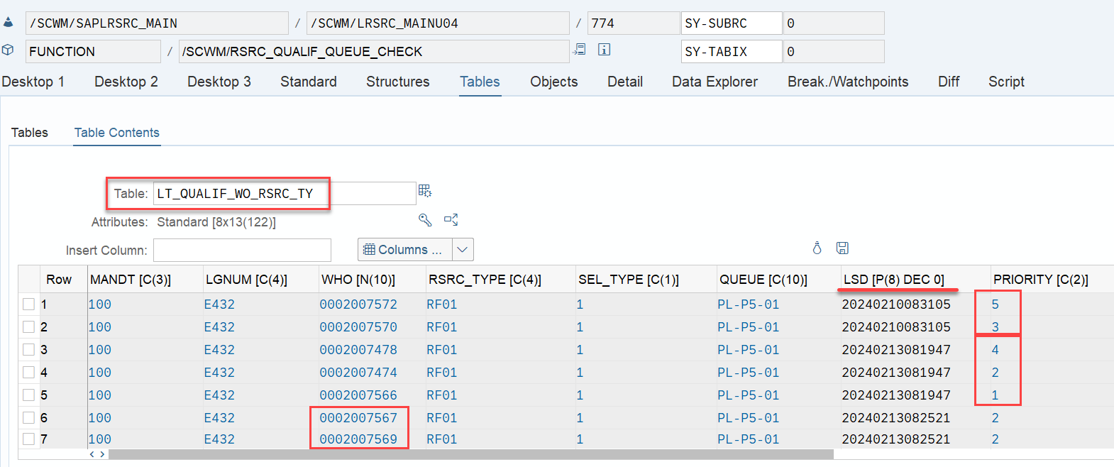
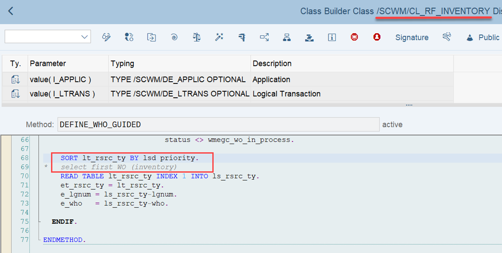
At the end, EWM just proceeds with the first WO from the list/table.

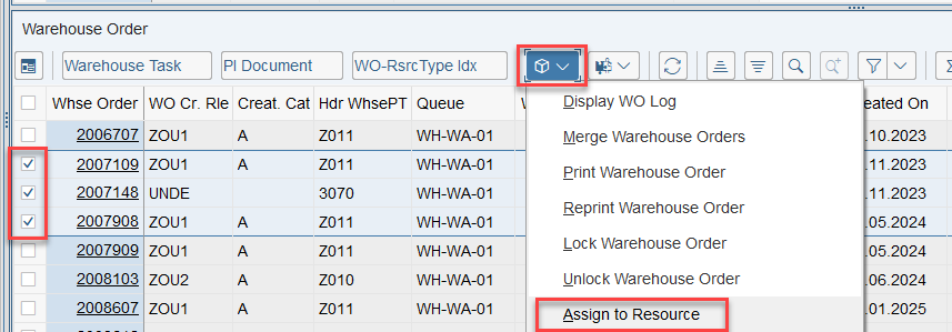
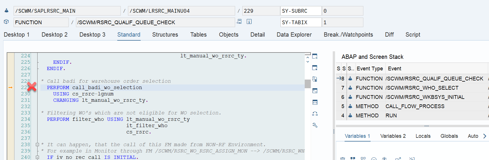
That was straightforward right!? This scenario however, is only executed if there are no manually assigned WOs. The latter is always checked one step earlier. Let’s assume a list of WOs has been manually assigned to the resource by the warehouse supervisor (e.g., via the warehouse monitor option, calling FM /SCWM/RSRC_WO_RSRC_ASSIGN_MON, which in turn calls FM /SCWM/RSRC_WHO_SELECT).


Assignments are read via FM /SCWM/RSRC_WHO_RSTYP_GET and, of course, always have a higher priority than non-assigned WOs. The sorting in this case – no surprise over here – is making use of the same ruleset that we saw before:

Options for enhancement

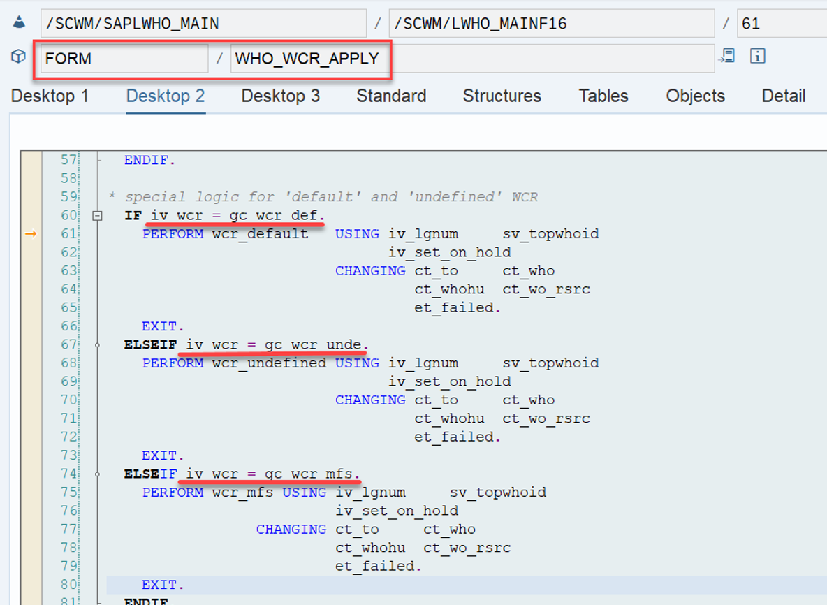
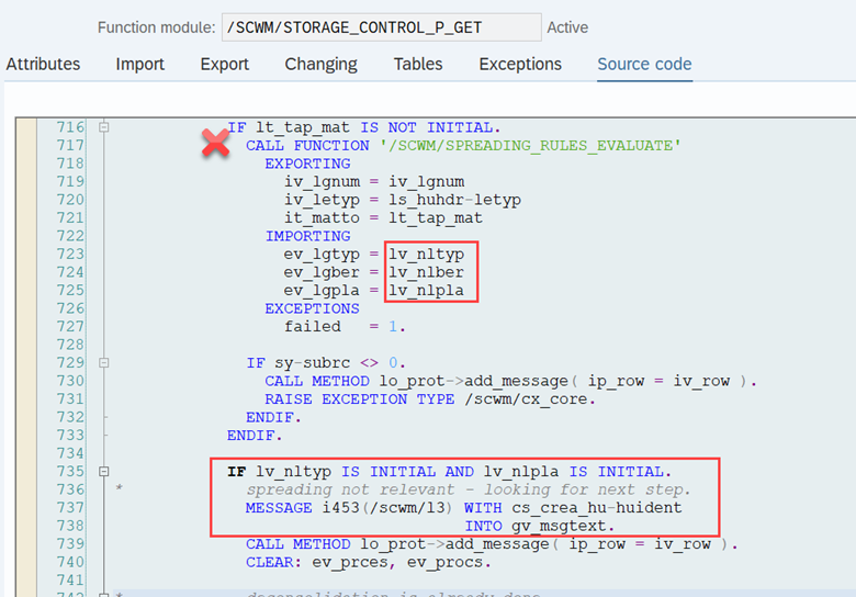
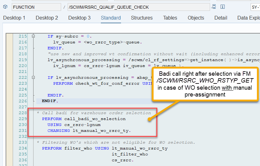
What is surprising though, is that EWM offers an option for a custom sorting in the pre-assignment context, which is not offered in the scenario where the WOs are not pre-assigned.

BAdi /SCWM/EX_RSRC_PROC_SEL
* With this BAdI you can influence the WO selection.
* You get the list of manual assigned WO’s and can
* resort them or
* delete WO from the list or
* return a new WO according your own selection (You must set LGNUM, WHO
* & CONTENT at least)

Question from a stupid EWM Consultant: Can somebody explain why this is BAdi not simply called in the same way in the non-pre-assignment context? If yes, please add your thoughts as a comment to the corresponding video!

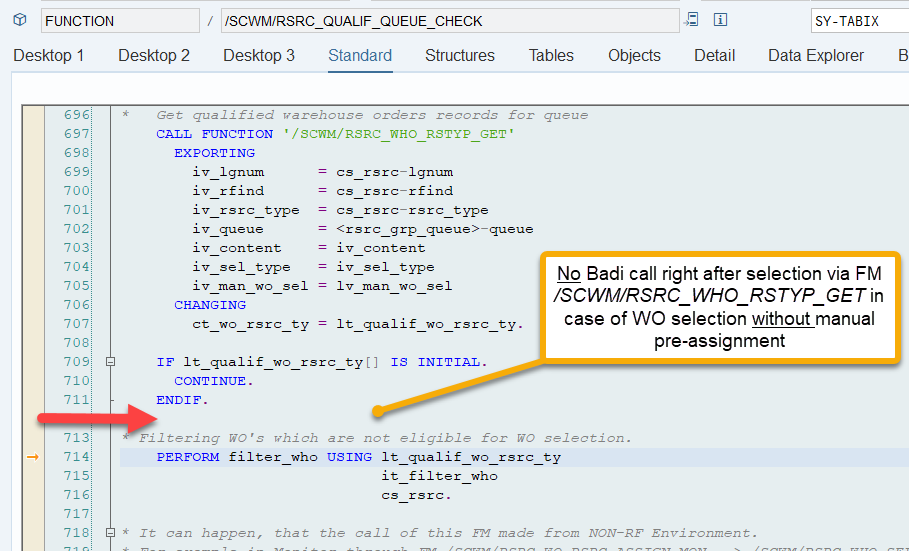
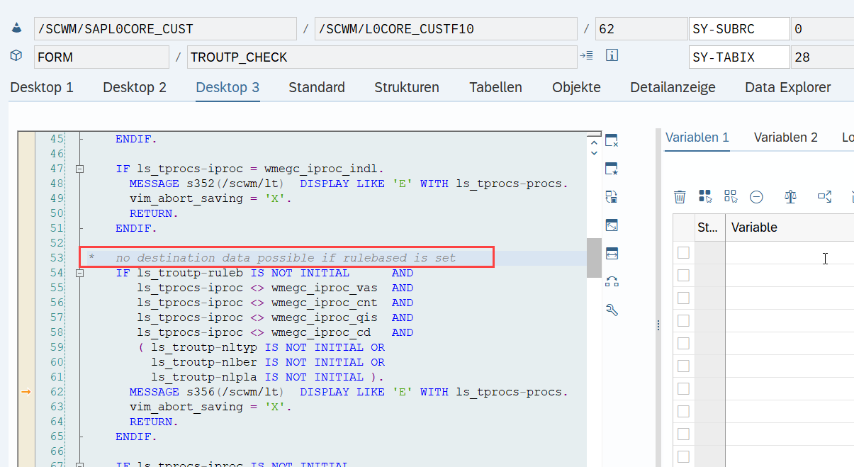
The filter_wo subroutine does not offer any option to manipulate the sorting here. Therefore, the only option to enhance the sorting is to intervene before the actual WO processing. You can include your own logic at the point when EWM creates the WOs and calculates the two values that are later used for sorting.

  • LSD: I explained the option to enhance the LSD in this video (video & blog-post).
  • Prioritization: The prioritization as the second sorting criterion can be manipulated via a custom logic using BAdi /SCWM/EX_RSRC_PROC_WO.

Fun facts / Party-knowledge

Sorting of WOs for physical inventory

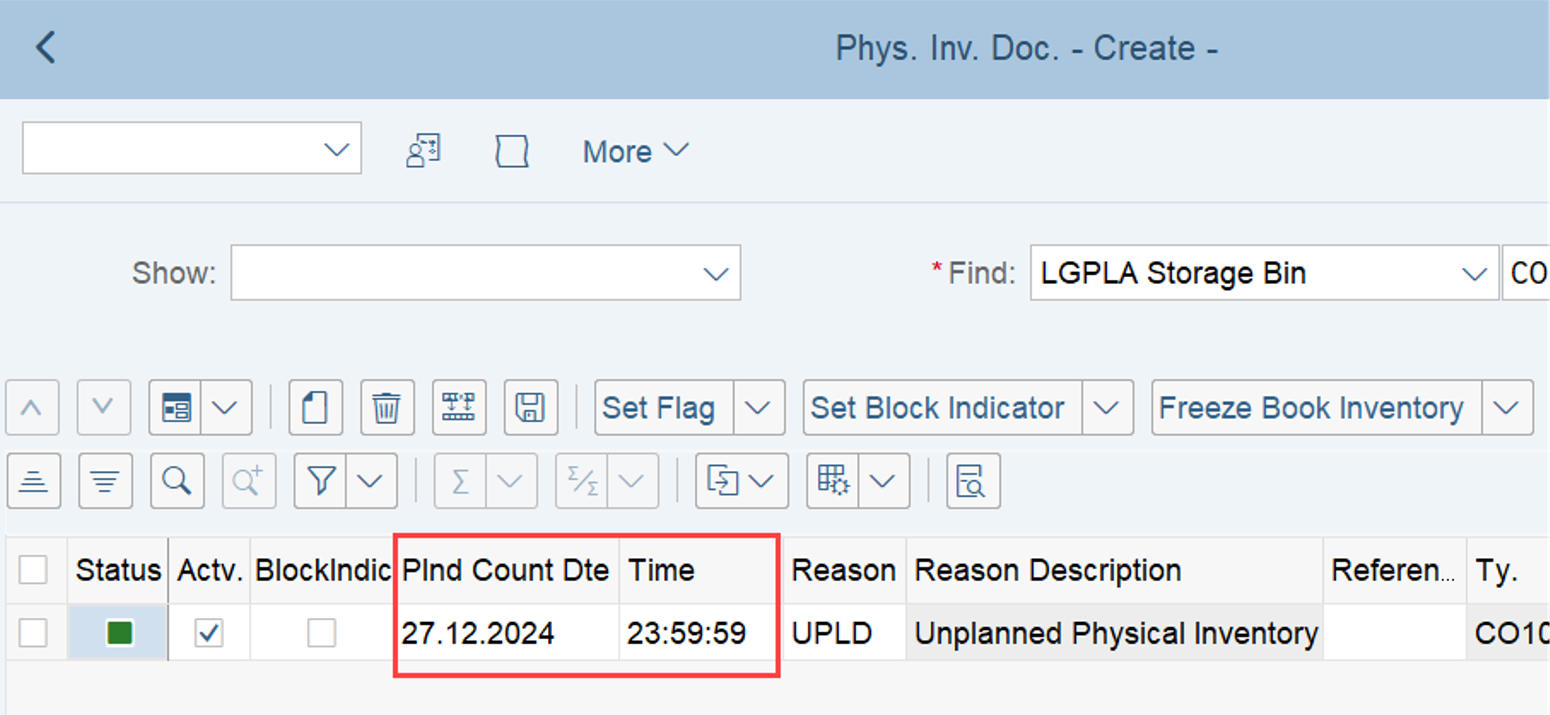
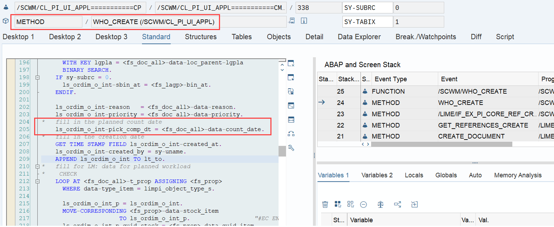
Nothing to reveal here. The sorting for PI WOs is based on the same criteria as for the normal WOs discussed above. As you learned in my campaign (video & blog-post) about the LSD calculation, for PI documents the LSD is derived from the planned count date. The priority is coming from the PI customizing.

Sorting in case of Task Interleaving

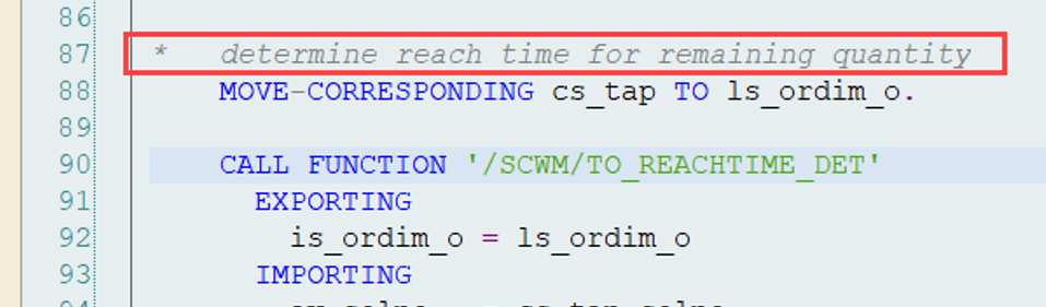
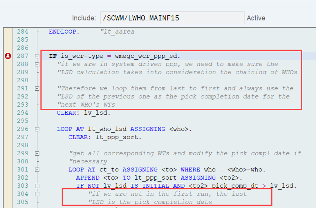
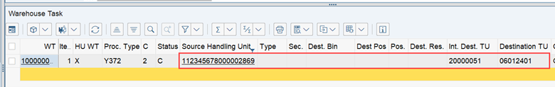
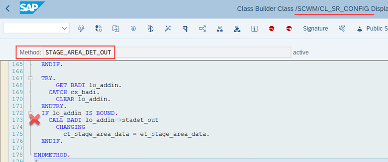
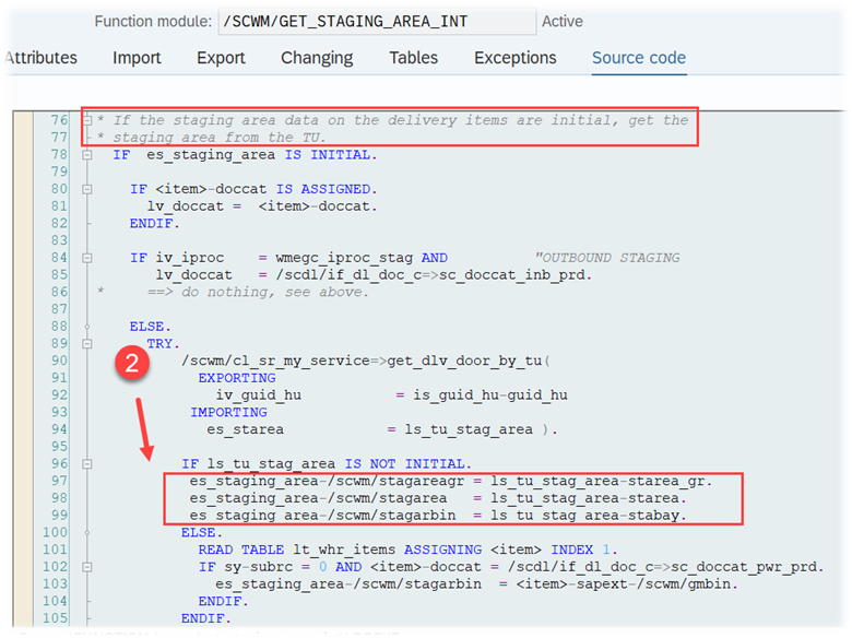
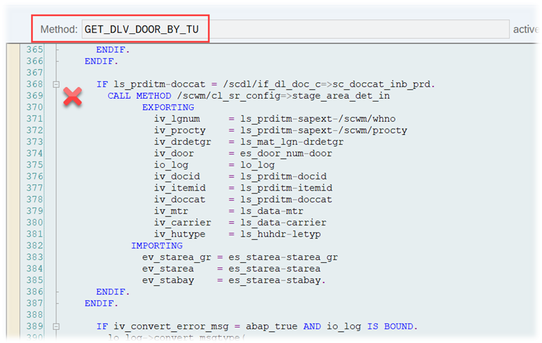
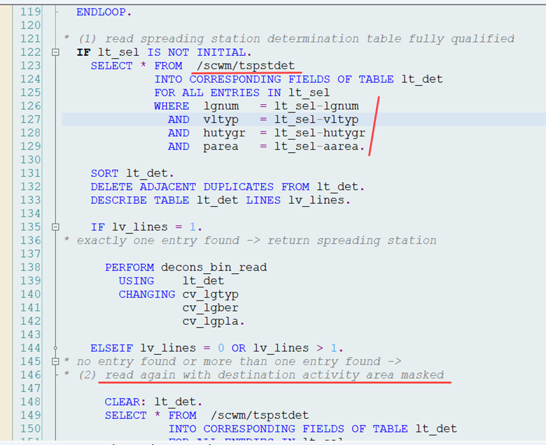
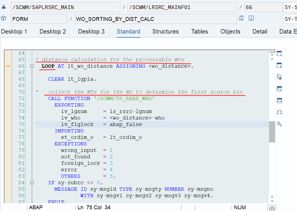
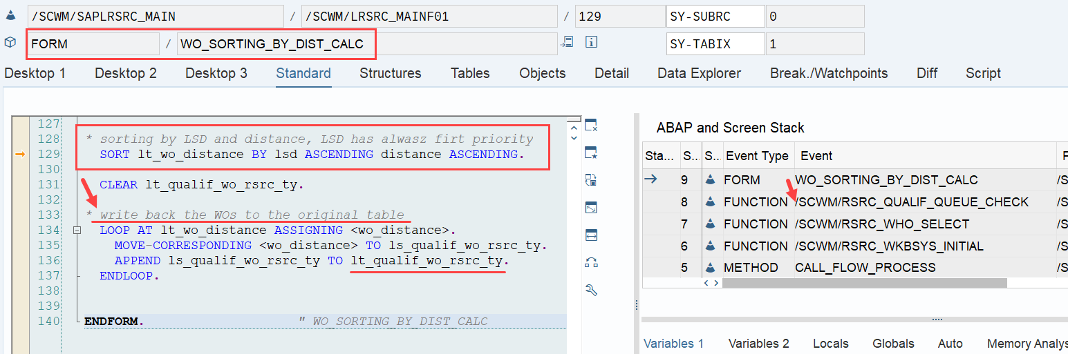
This is the most interesting part of this article in my opinion. If interleaving is active (refer to this video & blog-post if you are not familiar with the interleaving concept as such), EWM applies a slightly different logic for WO sorting, which I found only in the code (spent not that much time to browse all books to be honest). This occurs at the end of the function module FM /SCWM/RSRC_QUALIF_QUEUE_CHECK. Here, EWM considers the distance between the WOs instead of the priority used previously.

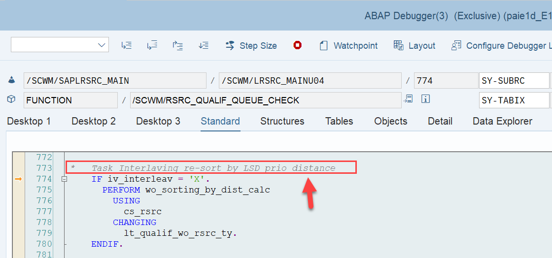
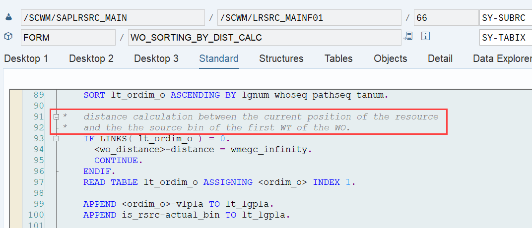
EWM loops over all WOs in the interleaving queue (~ the next queue from which it is supposed to pick a WO, based on the interleaving settings) and calculates the distances between the current position of the resource and the distance to the source bin of the first WT in every waiting WO in that queue:

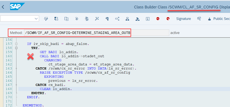
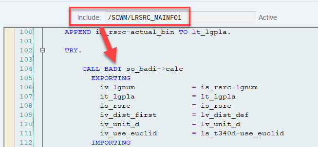
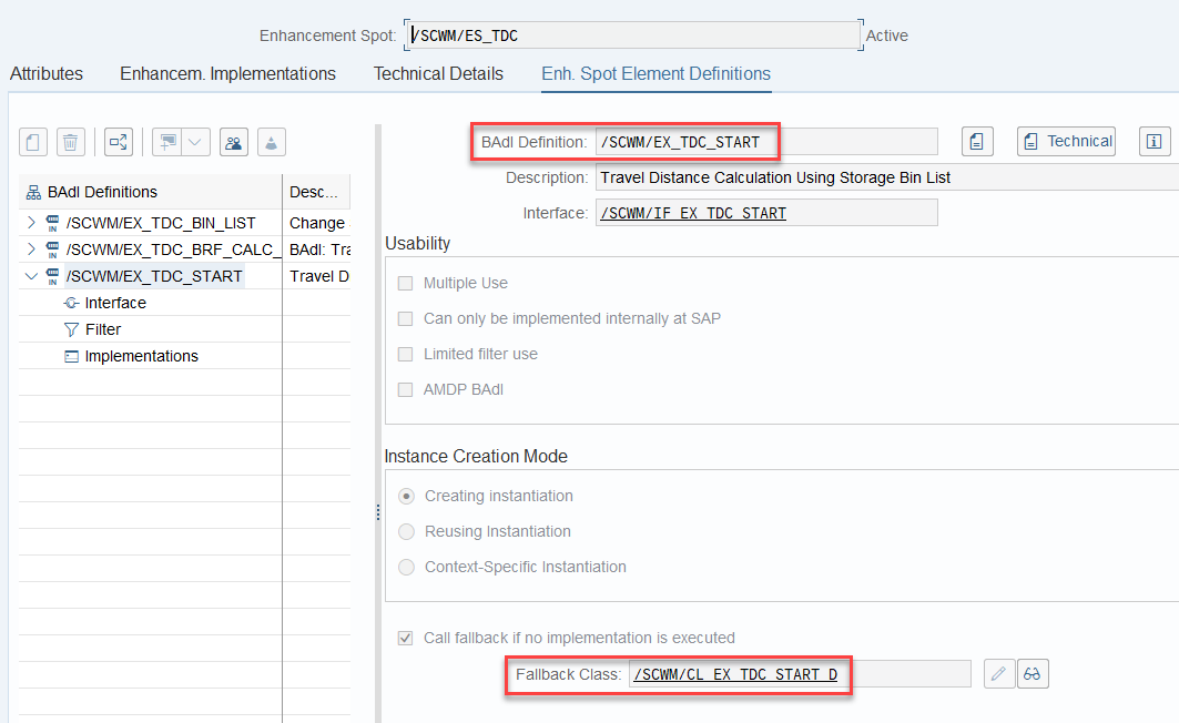
The distance calculation can be manipulated via BAdi /SCWM/EX_TDC_START. EWM itself calculates with the example/fallback class /SCWM/CL_EX_TDC_START_D of this BAdi (you should copy that class and use it as a base in case you want to include your custom logic here).

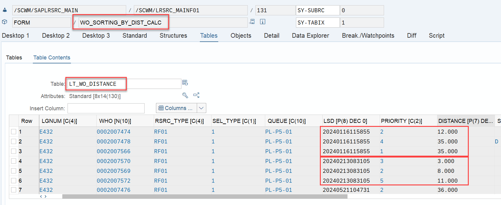
At the end can see that the LSD still has the highest value, but now the distance has a higher value than the ‘priority’ (which is no longer used in the context of interleaving).

A closing remark that I couldn’t overlook: I have great respect for the developers and I am forever grateful to have the opportunity to work with this software, but why the hell does a 300 billion company like SAP still ships software with so many typos in the comments of their code? Can’t the pretty printer check that as well? …or any kind of AI browsing through the code before it is being shipped?

Sorry… Back to our topic – 

The following example visualizes the approach for sorting during interleaving, that I explained above:

…and that completes the last subtopic that I wanted to address here. As usual, I will not let you go without a quick summary of the most important points. 

Summary

  • Sorting is the same with or without manual pre-assignment of warehouse orders to resources (1.LSD > 2.Priority > 3.WO number)
  • Only with manual pre-assignment the sorting can be changed in a clean and simple way (EWM offers a BAdi). Without manual pre-assignment, LSD and priority have to be manipulated during WO creation in order to implicitly change the sorting later
  • PI WOs are being sorted based on the same criteria as other WOs
  • In the context of task interleaving, the priority as a sorting criteria is replaced by the distance between the processing resource and the source bin of the first WT in the next WO

As we wrap up this blog post, I hope you found the information presented in a clear and digestible manner. While there may not have been many surprises, I trust that these last few minutes of reading have added to your EWM knowledge stack. Thank you for taking the time to read through!

Please feel free to subscribe to my blog updates or my youtube channel in case you want to be notified about new posts!

Get my monthly blog-updates!

Subscribe to my Youtube channel!

The post Reveal SAP EWM – Warehouse Order sorting in Queues appeared first on WMexperts.online.

By: Hendrik
22 March 2025 at 15:31

Reveal SAP EWM – Calculation of the Latest Starting Date (LSD)

Reveal SAP EWM

Calculation of the Latest Starting Date (LSD)

By reading this blog post, you will learn everything you need to know about how EWM calculates the Latest Starting Date for warehouse orders. Once again, I took a deep dive because I was not satisfied with the explanations I found in the SAP help texts. Here, I share the results of my analysis and, as usual, I promise to reveal some of EWM’s secrets. 🙂

What is it and what can it be used for?

Let us start with defining what the LSD actually is. In the 2nd part of this post, I will try a deep-dive into the calculation of the LSD. As you know it from my articles/videos, I promise to reveal some details and information that you will not fine in the SAP help or any of the SAP books! The latest starting date (LSD) is the latest point in time by which execution of a warehouse order (WO) should commence, so that it is completed by the due date & time. It is calculated on warehouse task level but saved for the warehouse order.

SAP help: The system calculates the LSD of a WO by: Calculating the LSD of each WT as described above Taking the worst-case scenario LSD (that is, the earliest LSD)

It is calculated in the context of resource management. Technically that means that it is only calculated in case the given WT found a queue with operating environment 2, 3 or 5:

Later during processing of the warehouse orders, the LSD is mainly used for sorting the WOs in the queues (this is true for the RF environment as well as for the MFS). Note that some other factors also have an impact here. We will not tackle the queue sorting further here but it is on my list for the upcoming months!

Examples for sorting in the RF and the MFS queues (standard MFS warehouse order selection for resources (e.g. high-bay cranes) is also sorting the WOs in the queues based on the LSD):

How to calculate and set the LSD?

Based on the SAP help text, the LSD is calculated as follows:

LSD = WO due date(planned execution duration + planned movements duration)

Simply imagine the ‘due date’ being one point in time in the future and interpret the minus (-) components as those time periods in which we need to move backwards from this point in the future in order to find our starting point.

This is the most important formula which will accompany us until the end of the article/video. In the following chapters we will try to break that down and analyse the different components.

Before we start our deep-dive, it is important to understand that the LSD is calculated for each possible resource type due to the fact, that the velocity of the resource type has an impact on the movement duration and therefore also directly on the LSD calculation. The final LSD for the WO is then the LSD for the slowest possible resource type. During WO creation we do not know which resource will later process the WO so we better assume the worst case and write the corresponding LSD into the WO.

FM /SCWM/RSRC_WHO_CREATE is the one to collect all resource types which are allowed to process the given queue (considering allowed HU type groups and allowed bin access types from customizing) and hands them over (along with the WO and its WTs) to our most important player: FM /SCWM/RSRC_LSD_CALC:

FM /SCWM/RSRC_LSD_CALC starts to collect the data to fill the variables for our formula shown above:

Based on this comment we have learned something new already. Our formula LSD = WO due date(planned execution duration + planned movements duration) Can also be written in a short form as: LSD = DD – (MOVE_DUR + PP_DUR) LSD = DD(MOVE_DUR + PP_DUR) What else did we learn from the comment above? DD: Seems to be coming from the wave header This brings me to the question about what we use in case we do not use waves? MOVE_DUR: Distance divided by resource type velocity This brings me to the question about how we actually calculate the distance? PP_DUR: Seems to be coming from the warehouse order creation This brings me to the question about how and where we calculate the pick and place duration? Let’s dig into detail, and answer those questions one-by-one! We start with the WO due date The due date is retrieved from subroutine get_due_date and is determined based on the different completion timestamps of the wave template or the planned departure from yard from warehouse request header:
Option 1: With wave management If maintained, EWM uses the pick completion timestamp from wave template as the due date. The pick completion date is written into the WT earlier in the stack at different places, depending on the way of creating the WT:

*Party-Knowledge*
If the pick completion timestamp is not set in the wave template option, EWM determines the storage process step that happens after the picking step (PACK in our example but it can also be staging or loading). From there it takes the planned duration and calculates backwards against the planned completion timestamp (from the wave template) of the corresponding step.


Example:

  • Pick completion is not maintained
  • Packing step is taking 10min (600sec) based on the POSC customizing
  • Pick completion = Pack completion – 600sec

(pls ignore the 1h time-shift between warehouse time and DB time in my system!)

If either

  • waves are not used at all
  • the pick completion timestamp is not maintained and you are not using storage processes / POSC
  • the pick completion timestamp is not maintained but also the completion timestamps for packing, staging and wave completion (loading) are initial

The due date is the planned departure from yard from the warehouse request header (which might be set by the ‘planned departure’ timestamp from the transportation unit in case you are using TUs).

Important note (again, a secret that is not mentioned anywhere in any of the SAP user manuals that I know) –
If maintained in customizing, EWM substracts from this planned departure also the duration of all POSC process steps that happen after the picking step. This makes a lot of sense as picking should not be completed when the goods leave the warehouse but rather at an earlier point in time to have some buffer left to pack, stage and load the goods:

For the sake of completeness –
The logic to set the due date for physical inventory warehouse orders is based on the planned count date, which can be provided during PI document creation (set in method /SCWM/CL_PI_UI_APPL-WHO_CREATE):

As the next part of our formula, we will look into the calculation of the execution duration.

planned execution duration (~ PP_DUR)
SAP help for the LSD formula (and comment in the code above)
The planned execution duration is taken from the WO

…that does not help much 🙁

EWM offers two main approaches to calculate the planned execution duration

  1. With Labor Management (the options to calculate the LSD via LM is not in scope of this blog post as it is quite complex and based on my experience most of you will probably not use it anyways)
  2. Without Labor Management the duration is retrieved in our LSD context in FM /SCWM/RSRC_LSD_CALC via the subroutine get_pick_place_duration (screenshot below)

The subroutine get_pick_place_duration however does not calculate anything. It simply reads the result from the WO data where it had been filled before based on customizing data from different places. Let us have a look at those places/components! To be honest, I cannot ensure that there are some components that I missed (the coding is quite complex here). I am sure I covered the most important ones. In general, you can imagine the calculation to work like this:

Execution Duration = Preparation time of the WO + Execution time of WT #1 + Execution time of WT #2 … + Execution time of WT #n

Preparation time: The preparation time calculation is pretty easy. The value can be derived from the WOCR that was used to create the WO (screenshot):

Execution time: The execution time is called ‘extract time’ in the customizing and ‘reach time’ in the coding/dictionary objects (SAP is again not very consistent with their wording here).

Both of them describe the time that the picker needs to grab the items from the source bin (and place it on the pick-HU) and to place it (from the pick-HU) to the destination bin.

It’s parameters & values are defined in customizing. For each movement (take from source or place to destination) you can define a constant time (e.g. to open the source box/HU/bin) plus a variable time depending on the quantity to be removed/placed. You can find the customizing path below along with an example setup that I created to simplify the understanding . Note that the F4 help for this customizing node is exceptionally detailed (worth is to read through). In short – you can define the constant as well as the variable part of the execution time depending on the UOM of the task, the product attributes, the bin access type and the WPT category. Quite a flexible framework!

The logic for the calculation is sitting in FM /SCWM/TO_REACHTIME_DET (final calculation in include /SCWM/LTO_REACHTIMEF04 via subroutine reachtime_det) where it is calculated for each WT for the source as well as the destination bin. In my example I made it easy and used the same time calculation for source as well as destination. This might not reflect the real world where placing at the destination is usually much faster than picking from the source (you could easily implement such a logic by using a different access type for the destination bin and set a lower or zero extract time based on this). Time calculation for the source bin movements + time calculation for the destination bin movements:

The following screenshot summarizes the result with the objective to make it understandable for everybody.

(1) Preparation time from WO customizing
(2) Extract/Reach time calculation for each WT from ‘Define Extract Time Determination’ customizing
(3) Extract time calculation for each WT (sum for source and destination extract times)
(4) Total time on WO-level (preparation time + extract time of all WTs)

I think based on this, everybody understands now how EWM calculates the planned execution duration which is used as part of our LSD calculation formula! Note that there are a lot of details and options to calculate the execution time that I did not mention here at all. I only gave you a rough overview to help you understand it as a component which is used for the LSD calculation. For a deep-dive of the execution time calculation I will drop another post/video within the next months. Next stop! Last but not least, let us have a look at the 3rd part of our formula. The planned movement duration. planned movements duration SAP help The planned movements duration is equal to distance/velocity. The following rules apply here: Distance is calculated according to the bins’ coordinates, using the manhattan metric Velocity is the lowest horizontal velocity from all resource types that are qualified to execute the WT Let’s see. We need to calculate travel distance & time now. Again, we assume that Labor Management is not active so we cannot use the numbers being returned from LM. Still, EWM offers two different options to calculate the movement duration:

Option 1 (the old ‘Travel Distance Calculation’): The 1st option is the ‘old’ (and default) way of calculating based on the X & Y coordinates of the bins. The logic is sitting in FM /SCWM/BIN_DIST_GET which is called by subroutine get_travel_distance:

Option 2: The ‘new’, more complex approach for Travel Distance Calculation. This one is based on method /scwm/cl_tdc-get_time_for_lsd and needs to be activated in the warehouse number settings.

I will not go into detail how method /scwm/cl_tdc-get_time_for_lsd calculates the distance. It is using some fancy algorithm for the distance calculation of the vertical and horizontal movements. Something we could spent another hour on together – maybe in a separate blog post… The main differences:
  • Option 2 offers a more sophisticated algorithm for the calculation (which I did not explore in detail and is not in scope of this article). Both will only work in case coordinates are maintained for the storage bins!
  • Option 2 offers many different Badis/entry points to change the standard calculation or create a custom logic for the distance calculation. Option 1 does not offer any possibility to include a custom logic
  • Option 2 calculates the travel time right away (considering the velocity of the slowest resource type) whereas option 1 calculates only the distance
We will not go further into detail here. Keep in mind that if you have maintained the bin coordinates they will be used for the calculation of the movement duration. If you haven’t done that, both options will not be able to return anything. No matter which option you choose, under consideration of the resource types velocity, the result becomes our planned movements duration which we need for our formula (again – technically with calculation option 2 above, the velocity is considered right away to calculate the travel time and with option 1 we EWM only calculates the distance and the velocity is considered in the next step described below).

Note that the customizing for Define Planned Duration of Movements in Warehouse does not have any impact on the LSD calculation, based on my research. Did not explore any other usages but seems SAP is only using this as a simplified option to calculate the planned completion timestamps for WTs in case you are neither using warehouse requests, nor waves. So not really interesting for us here.

With that, we now we have the required values for all variables of our formula: LSD = WO due date(planned execution duration + planned movements duration) Thus, the remaining step is the calculation of the LSD and the modification of this timestamp in the WO table for all resourse types. And this is how it looks like in detail:

The subroutine modify_lsd first calculates the travel time in case we used option 1 (mentioned above) for the travel distance calculation. It does this based on the distance calculated via FM /SCWM/BIN_DIST_GET (remember option 1 mentioned above) and the velocity of the different resource types. As mentioned, this is only required in case the travel time calculation has not yet happened via method /scwm/cl_tdc-get_time_for_lsd and handed over to our subroutine (remember option 2 for travel time calculation mentioned above).

The result is added to the execution duration (pv_plandura_sec in the screenshot below), that we got above from subroutine get_pick_place_duration above. The sum results in the total duration (movement duration + execution duration):

Note that if labor management is active, the travel duration is already part of the planned duration coming from LM and not calculated again here.

Once the total duration is calculated, FM /SCWM/RSRC_TIMESTAMP_SUBTRACT finally executes our main formula. It uses the total duration to calculate backwards based on the due date. This finally delivers the LSD:

This LSD is then saved for all allowed resource types in table /SCWM/WO_RSRC_TY and once for the WO in table /SCWM/WHO:

And with that we have reached the goal of this blog post. We have calculated the LSD and and understood every component of the formula it is based upon:

LSD = WO due date(planned execution duration + planned movements duration)

Note that SAP offers an option to manipulate the results of calculations without any coding (thanks to Jelle Verhagen for pointing that out!!). Rounding rules can be determined based on the activity or wave template. For example, you can equalize all LSDs calculated for a specific hour or day based on these rounding rules, limiting the WO sorting for this timeframe to priority and WO number only.

To achieve this, you need to define modes and the corresponding determinations based on the activity:

The result of the customizing shown above should not surprise you:

Works in a similar way for other rounding intervals – no further examples here :-):

In the example above, the mode for the rounding rule was determined by the activity of the warehouse tasks. If you are working with waves, as mentioned before, the mode assigned to the activity can be overruled by the mode that you assign to a wave (coming from its wave template option).

…and that finally concludes the main part of this article! 🙂

Last but not least, I would like to close this post with a tiny bit of party knowledge in the context of special scenarios, that did not really fit into the agenda so far 🙂

PMRs
I did not find any standard logic for the LSD calculation in the context of production integration using PMRs as warehouse request documents. This is mainly due to the due date not getting any input from the planned departure or wave templates. I will soon release a video about how to enhance the LSD calculation, which will also cover this scenario. Let me know in the comments in case you found a standard logic to calculate the LSD for staging WOs against PMRs!

Note that SAP recently announced to enable wave management also for PMRs, which might come along with the option to use the time-stamps from the wave templates also here!

Pick & Pass system-driven
When you use a WOCR where EWM decides about the sequence of the pick&pass, it also considers the duration of the chained WOs to calculate the pick completion dates and thereby the LSD for each sub-WO (this is pretty smart):

This summary marks the end of this post. As usual, I hope I could add some value for some or the other.

To finally wrap it up –

The LSD that we calculated above for a given WO, can easily be changed via the warehouse monitor manually:

This is easy but what can you do in case you want to calculate it right away based on a custom logic. Stay tuned for my next video. Smash the subscribe button and sign in for my newsletter so you cannot miss it!

Please feel free to subscribe to my blog updates or my youtube channel in case you want to be notified about new posts!

Get my monthly blog-updates!

Subscribe to my Youtube channel!

The post Reveal SAP EWM – Calculation of the Latest Starting Date (LSD) appeared first on WMexperts.online.

By: Hendrik
1 February 2025 at 10:17

Reveal SAP EWM – Warehouse Order Creation Rules DEF and UNDE

Reveal SAP EWM

Warehouse Order Creation Rules DEF and UNDE

Who hasn’t faced this situation before? You create a warehouse order, and EWM tells you that it used the warehouse order creation rule ‘DEF’ (or ‘UNDE’). And you’re like, “What the hell!?”
This blog post will help you avoid this situation in the future. It will also help you understand that sometimes seeing one of these two WOCRs is a signal to fix an issue in your customizing, and other times it might be just fine.
A minimal intro for those of you starting your journey with EWM:

A ‘Warehouse Order’ bundles multiple ‘Warehouse Tasks’ into processable work packages. The rules for this bundling process are called ‘Warehouse Order Creation Rules’. In the following, I will also use the abbreviation WOCRs to replace the long term.

For those of you who are not familiar with how the WOCRs work in general, I would recommend to read this blog before reading/watching this one here.
Adding a small summary here, which you can skip in case you are familiar with the concept (source SAP HTG for WHO enhancement): 

(1) Warehouse tasks are created in the system (for example, manually or by wave release).
(2) (3) The system groups the warehouse tasks by queue and activity area, and determines possible warehouse order creation rules according to the settings made in the Customizing activity Define Search Sequence of Creation Rules for Activity Areas.
(4) The system tries to apply the warehouse order creation rule according to the sequence specified in the Customizing activity Define Search Sequence of Creation Rules for Activity Areas.
(5) The system sorts all the warehouse tasks based on the inbound sorting criteria of the warehouse order creation rule.
(6) (7) At this stage, the system checks whether the sorted warehouse tasks pass the filter of the warehouse order creation rule on item level and on subtotal level.
(8) The warehouse tasks that have passed the filters are considered when applying the limits specified in the warehouse order creation rule.
(9) All the warehouse tasks that belong to one warehouse order are passed for packing proposal determination according to the packing profile of the warehouse order creation rule. As a result of the packing proposal determination, the system determines the creation of pick-HUs, the splitting of warehouse tasks (for example, to fit in a pick-HU), and the exclusion of warehouse tasks from the current warehouse order.
(10) Finally, the warehouse tasks that belong to the current warehouse order are sorted according to the sorting rule of the warehouse order creation rule.

After all the warehouse tasks have been checked against the warehouse order creation rule, the warehouse tasks that have not been bundled are checked against the next warehouse order creation rule defined in Customizing.

Anyways – back to the initial question.

What are those DEF and UNDE WOCRs and why are they sometimes applied when creating WOCRs?
First a quick look into the standard customizing help text:

We recommend that you avoid using the following abbreviations to identify warehouse order creation rules, since we have already assigned them internally for existing warehouse order creation rules. This ensures that the identification you define for a warehouse order creation rule is unique.

  • DEF: Standard rule
  • UNDE: Remainder rule

…ok – that does not help us at all.

Another look into the SAP Press functional EWM books:

  • If no warehouse order creation rule is set up in embedded EWM, it assigns all warehouse orders to default rule DEF.
  • If there are no more warehouse order creation rules left in the sequence for a warehouse order, the system assigns them to default rule UNDE.
    …that goes into the right direction abut also comes with a very limited amount of details.

The most helpful content that I’ve found over the years was this extract from the HTG for developers, working with WOs: ‘How To Program Warehouse Order Processing in Extended Warehouse Management’:

If a warehouse task doesn’t fit to any warehouse order creation rule, it’s bundled with the rule Undefined (UNDE), together with all the other warehouse tasks that don’t fit to any warehouse order creation rule.
If the system can’t find a warehouse order creation rule for an activity area in Customizing, the warehouse tasks are bundled with the warehouse order creation rule Default (DEF). This means that all the warehouse tasks for one delivery are bundled together if they are in the same activity area, except for the putaway warehouse tasks where the system creates one warehouse order for each putaway-HU warehouse task (fields FLGHUTO = X and TRART = wmegc_trart_put (1)).

Why do I have to search for this information in the HTG for developers? Why is it not included in the customizing help text?

Anyways – I still had some open questions, and the same is probably true for you. So, let us look into the system to see if we can find more details about this logic. As usual, I found some useful details that are not included in any of the SAP documents mentioned above!

While trying to structure this post, I decided to start by looking at the application area of the WOCR ‘DEF’, first in the context of putaway and internal tasks, and then in the context of stock removal. In the second part of this post, we will concentrate on the WOCR ‘UNDE’ and again separate it by process category (putaway vs. removal).

Throughout the whole article, I am working with test cases and examples to help you understand my findings. In addition to this, you will also find all repository objects that are responsible for controlling the logic.

ANALYSING the WOCR ‘DEF’

At first we want to understand the purpose of the WOCR DEF in detail. Remember, the HTG gave us the following information:

If the system can’t find a warehouse order creation rule for an activity area in Customizing, the warehouse tasks are bundled with the warehouse order creation rule Default (DEF). […] except for the putaway warehouse tasks where the system creates one warehouse order for each putaway-HU warehouse task (fields FLGHUTO = X and TRART = wmegc_trart_put (1)).

So, we start to analyze the behavior of the EWM standard in a situation where it cannot find any WOCR based on the given combination of activity area and activity. Let’s look at putaway and internal movements first, before we explore stock removal.

PUTAWAY/INTERNAL MOVEMENTS

I start using a warehouse process type of category ‘1’ (putaway) and removed the WOCR determination customizing for my given combination of AA and Activity. The only ones left for my AA were relevant for a different activity:

The coding which is responsible to apply WOCRs is called from FM /SCWM/WHO_PARALLEL_CREATE. Based on my customizing, it cannot find a WOCR for the given AA/activity and proceeds with the ‘special logic’ (trying to apply rule MFS or DEF). As our tasks are not relevant for a subsystem (rule ‘MFS’), the only option left is to hand over the constant for the rule DEF to the subroutine who_wcr_apply.

If we are talking about HU WTs of the type ‘putaway’ (WPT TRART = ‘1’ > see WPT customizing screenshot above), this subroutine will make sure to always create a separate WO for each WT.

For our putaway example that means one WO for each HU WT which is created with a WPT of category ‘1’:

And this is the result:
Double-checked with multiple HU-WTs, running through the WOCRs at the same time. Even if they are going to the same destination, EWM will create separate WOs:

Main takeaway? or What does that mean for you?

If you are

  • working with handling units as part of the inbound process
  • and you have a simple putaway step/process
  • where you want to create one warehouse order for each HU to be putaway

…it is totally fine not to create any custom WOCR at all. You can keep the customizing lean at this point and work with the standard default (DEF) rule.

But again – this is only true if you are working with HU WTs and if your WPT is of type ‘putaway’. Once you switch to product WTs or WPTs of type internal movements (e.g. for replenishment) EWM still applies the DEF rule if it does not find a WOCR but it does not apply the logic to split the WTs into a 1-1 relationship within the WOs. As the screenshot below shows, we have now a 1-n relationship between WO and WT:

Putaway done! When and how does the DEF rule behave in the context of stock removal?

STOCK REMOVAL
Remember what the HTG told us

[…]This means that all the warehouse tasks for one delivery are bundled together if they are in the same activity area

Let’s try to find the logic behind!

Without any WOCR for the given combination of activity area and activity we are ending up with the same FM calling the same subroutine with the same constant as we saw it in our example for the putaway task creation. Subroutine wcr_default is the one that makes sure that warehouse orders do only receive tasks from one combination of activity area, queue and delivery / reference document / warehouse request:

Not much more to see here to be honest. The result is as expected:

Main takeaway? or What does that mean for you?

If you are working with warehouse requests (e.g. deliveries) and you do not have any specific requirement apart from

  • creating one single warehouse order for all warehouse tasks of a single warehouse request
  • which are removing stock from the same activity area
  • and are assigned to the same queue

…you do not have to configure a custom warehouse order creation rule for that but can keep it lean and work with the EWM standard default (DEF) rule.

First part done. I think that was straightforward and easy to understand! Let us now have a look at the WOCR UNDE!

ANALYSING the WOCR ‘UNDE’

The HTG gave us the following information for this scenario:

If a warehouse task doesn’t fit to any warehouse order creation rule, it’s bundled with the rule Undefined (UNDE), together with all the other warehouse tasks that don’t fit to any warehouse order creation rule.

That is not a lot of details and as you can see further below, this is not 100% true. Anyways – we now want to analyse the behavior of the EWM standard in a situation where it indeed finds a WOCR for the given combination of activity area and activity but it cannot apply this rule (e.g. because the WTs did not pass the item filter).

Same as before, we first have a look at putaway and internal movements, before we explore the stock removal.

PUTAWAY
For this example I created a WOCR for the given activity area / activity but set the item filter in a way that our WTs would not pass it:

The relevant spot in the coding is the same as before where we ended up with rule ‘DEF’. Again, FM /SCWM/WHO_PARALLEL_CREATE tries to apply the WOCRs. In the scenario we are looking at now, it actually finds one WOCR for the given AA/activity (see internal table lt_twcrsseq):

Subroutine who_wcr_apply first tries to apply one of the WOCRs to the given WTs. As this fails, the FM proceeds with the ‘special logic’, trying to apply MFS or UNDE). As our tasks are not relevant for a subsystem/MFS, the only option left is to hand over the constant for the rule ‘UNDE’ to the subroutine who_wcr_apply, which then calls subroutine wcr_undefined:

The comment in subroutine wcr_undefined gives us a better understanding about what to expect:

* So-called “undefined” warehouse order creation rule that will be
* processed if all rules of a the activity area have been processed
* and there are still TOs, which were not bundled.
* This rule creates one bundle per dstgrp (in an activity area and
* queue).

@SAP Why can’t we have such details in the help text for the WOCR customizing? 🙂

Based on this we expect to end up with one WO for each combination of activity area, queue and distribution group. Note that in the context of putaway the term ‘distribution group’ refers to the deconsolidation group which can be assigned to the bins based on the activity area (sitting in table /SCWM/LAGPS):

As expected, as a result of our test we end up with one WO which is created with WOCR UNDE, carrying all WTs for which EWM could not apply one of the WOCRs from customizing. Even HU WTs of type ‘putaway’ are now combined in one WO (which is different to what we saw with WOCR ‘DEF’):
Once I use different distribution groups for the different destination bins, the result looks like this (in the example I used one bin with and one without distribution group):

…this is the 1st point that I had in mind when I said the text in the how-to-guide is not 100% correct. As in fact, this is not happening: “it’s bundled with the rule Undefined (UNDE), together with all the other warehouse tasks that don’t fit to any warehouse order creation rule”.

Note that EWM does not make a difference here between putaway or internal movements. No special rules apply based on the WPT category (like we saw before with the ‘DEF’ rule).

STOCK REMOVAL

In a similar situation during stock removal, the call stack looks exactly the same. Subroutine who_wcr_apply fails to successfully apply one of the WOCRs to each of the given WTs and FM /SCWM/WHO_PARALLEL_CREATE proceeds with the ‘special logic’ (trying to apply WOCR MFS or UNDE).

As our tasks are not relevant for a subsystem (rule ‘MFS’), the only option left is to hand over the constant for the rule ‘UNDE’ to the subroutine who_wcr_apply, which then calls subroutine wcr_undefined. For stock removal we can find a split logic similar to the one that we saw for the putaway scenario above. Independent from the WOCR logic discussed here, EWM fills the distribution group field in the WT with the consolidation group of the warehouse request item. For us this also means that the WOCR ‘UNDE’ will split by default based on this consolidation group for removal tasks (in the same way as it split based on the distribution group during putaway). In the context of stock removal the term ‘distribution group’ refers to the consolidation group which can be assigned the warehouse request items.

Example with a single consolidation group:

Example with two different consolidation groups:

…this is the example that I had in mind when I wrote that the statement from the how-to-guide is not 100% true:

If a warehouse task doesn’t fit to any warehouse order creation rule, it’s bundled with the rule Undefined (UNDE), together with (!!) all the other (!!) warehouse tasks that don’t fit to any warehouse order creation rule.

Summary

Unfortunately the help text included in the customizing does not help much here and also the functional books from the SAP press do only provide an absolute minimum of technical details. The HTG for WO enhancements gave us a good picture but again, a comprehensive understanding of how and why EWM applies the WOCRs DEF and UNDE could only be gathered based on a code-review.

Key points that you should take away from this blog post:

In case you do not define any WOCR at all for the given combination of activity area and activity, EWM applies the special rule ‘DEF’

  • For HU WTs created with a WPT of category ‘1’ (putaway), EWM creates a dedicated WO for each WT
  • For product WTs or any other kind of WPT category, EWM creates one single WO for all such WTs in the given warehouse order creation run
  • For stock removal WTs, EWM creates one WO per AA & queue for each delivery

In case you have defined WOCR(s) for the given combination of activity area and activity but the WTs cannot be processed by those WOCR(s) (e.g. do not pass the filters), EWM applies the special rule ‘UNDE’

  • In the context of putaway, separate WOs are created based on activity area, queue and the distribution group of the destination bin
  • In the context of stock removal, separate WOs are created based on activity area, queue and the consolidation group of the corresponding warehouse request items

For those of you who want to explore further details about the standard coding, the subroutine who_wcr_apply might be the most straightforward entry point:

This summary marks the end of this post. As usual, I hope I could add some value for some or the other.

In any case, thanks for spending your time to read this stuff! Enjoy learning and visit my blog again from time to time!

Please feel free to subscribe to my blog updates or my youtube channel in case you want to be notified about new posts!

Get my monthly blog-updates!

Subscribe to my Youtube channel!

The post Reveal SAP EWM – Warehouse Order Creation Rules DEF and UNDE appeared first on WMexperts.online.

By: Hendrik
2 November 2024 at 01:39

Reveal SAP EWM – Storage bin sorting during putaway (CLSP)

Reveal SAP EWM

Storage bin sorting during putaway (CLSP)

This blog is supposed to clear up one of the biggest misconceptions in the context of bin determination during putaway task creation in SAP EWM.

Before we jump into the system, let us quickly make sure to understand the scenario from material flow / process perspective –
Imagine you want to putaway a handling unit – let us assume a pallet loaded with some cartons – into a pallet rack. You have defined a strategy to determine an empty bin. All bins have the same bin type. So far so good. However, there might be lots of empty bins in the given rack. So how should EWM now decide which bin to suggest for the putaway process?

At this point, the bin sorting comes into the game!

I will explain the topic for you based on the following agenda:

  • The standard logic
  • The configuration
  • The bin sorting
  • The coding
  • Options for enhancement

As a starting point it is important to understand that whenever EWM is sorting something based on storage bins (e.g. warehouse tasks within warehouse orders, bins during putaway etc.) it is using so called ‘sort sequence numbers’. Those numbers are assigned to storage bins. EWM never uses those sequence numbers alone. It usually uses a combination of a sequence number along with an activity area and an activity type. Different combinations of activities, activity areas and sequence numbers can be attached to storage bins. Either based on the execution of a report (which is reading the sorting logic from the customizing) or based on an excel upload file.

The result with both options is saved in table /SCWM/LAGPS. I highlighted the important fields within the screenshot below:
The following activities can be used to attach a sort sequence number to a storage bin in EWM standard:
Based on this it seems to be obvious to sort bins based on the activity type ‘PTWY – Putaway’ in order to sort bins for the putaway process scenario described at the beginning of this post. Far from it! The sequence numbers assigned to the bins for activity type ‘PTWY’ is only used for the sorting of putaway warehouse tasks within warehouse orders (e.g. for travel path optimization in case you assign multiple warehouse tasks for putaway to one warehouse order). It is not used to sort bins during the actual determination of the destination bin. EWM indeed uses the sequence number for this activity type during putaway task creation but only after the destination bin has already been determined (we will come back to this point later again!). So if it is not the activity type PTWY, what else is being used in order to sort the bins during the destination bin determination for our example above? The answer to this question is the assignment of the combination of sort sequence numbers, activity area and the activity type ‘CLSP – Cross-Line Stock Putaway’ to the given bins.

The configuration

The creation of the activity area and its sorting can be done here:

  • Define an activity area via SPRO: SCWM Extended Warehouse Management -> Extended Warehouse Management -> Master Data -> Activities Areas -> Define Activity Areas
  • Then assign this Activity Area to storage type. Path in SPRO: SCWM Extended Warehouse Management -> Extended Warehouse Management -> Master Data -> Activities Areas -> Assign Storage Bins to Activity Areas
  • Then define sort sequence for CLSP Activity. Path in SPRO: SCWM Extended Warehouse Management -> Extended Warehouse Management -> Master Data -> Activities Areas -> Define Sort Sequence for Cross-Line Stock Putaway
Here you can now provide a logic for the assignment of the sequence numbers for sorting. For aisle, stack, level and subdivision you can decide whether you want to sort ascending or descending as well as whether you want to alternate or not. An example for the sort sequence between the 3 parameters is visualized in the screenshot below. Here I sorted 1st based on the stack and 2nd based on the level. You can see that EWM will first assign sequence numbers to all stacks of a given level before it proceeds with all stacks for the next level. This screenshot also shows how the ‘alternating’ approach is supposed to work. You can see that EWM counts the stack up until the max value and then decreases again from there for the next level. When you set this to ‘not alternating’ it would start again from the lowest stack value:
Here another example where I sorted 1st based on the level and 2nd based on the stack:
For all activities other than CLSP, EWM is sorting the aisles one-by-one. Only for CLSP it always sorts based on the aisle first. Another example to help you understand this approach along with the options for alternating:
Note: If you leave all other fields blank, the system simply sorts in ascending order based on the storage bin names. In addition to this, you have a parameter to fix the sorting. You can use this checkbox to ensure that the sorting is not changed during picking with radio frequency (RF). If you select this checkbox, it is not possible for the operator to change the path sequence during picking.
And that is it for this post! Pretty sure most of you are already using one or the other tool that I presented here. I hope that some of you still found something new here that helps you during your daily tasks in the future!

The bin sorting

Once the customizing is completed as shown above, the bins have to be sorted via transaction /SCWM/SBST:

Once the sorting has been executed, the sequence numbers are saved in table /SCWM/LAGPS as well as /SCWM/LAGP. This is also different compared to other activities where the sorting is only saved in the LAGPS table. Could not find the reason why we have it in two tables honestly. Maybe anyone has a good idea!?

The coding

It is interesting to observe that the although activity CLSP is not given as activity type in the customizing of the warehouse process type, it is still used for the sorting in our scenario:
Seems SAP noticed at some point that the WPT parameter is required for the activity which is used for the sorting within the WO (mentioned at the beginning of this post) and thus, needed a different approach to determine the sequence for the bin selection. For non-MFS storage types the sorting is done in include /SCWM/LPUT_BIN_DETF77, subroutine SORT_EMPTY_BINS, right after a list of possible destination bins had been determined via the subroutines BIN_DETERMINATION_1 & *2 in include /SCWM/LPUT_BIN_DETF17/ /SCWM/LPUT_BIN_DETF26. This is at least true for the empty bin determination. I have to admit that I did not spend time on analyzing the exact spot for addition to stock. However, I am pretty sure the function module which is finally used for the actual sorting is the same for both cases (so if you want to debug your specific strategy, just put a breakpoint into this one): /SCWM/ACT_AREA_EVALUATE
The FM imports the table of unsorted bins, reads the bin sorting against the imported activity type from the tables listed at the beginning of this article and exports a table with the same bins sorted accordingly:
…to be honest – I do not understand why the standard is coded like this. In line 26 it uses a constant to set the activity for our context. Then it fills lt_lgpla_unsorted from imported table IT_ILAGPL just to sort lt_lgpla_unsorted within the FM /SCWM/ACT_AREA_EVALUATE based on activity CLSP. However, the internal table that was imported to our subroutine here already had the field CLSP_SORT:
So why not just sort table IT_ILAGPL based on this field in line 32 ff. and return from the subroutine instead of calling FM /SCWM/ACT_AREA_EVALUATE? A big beer on my bill for anyone who can explain to me why this would not work! The logic for MFS storage types is less complex. Method /SCWM/CL_CORE_PUTSTRA-DET_EMPTY_BIN sorts the internal table of bins. As mentioned above, the field CLSP_SORT already exists in the LAGP table and here EWM does what I suggested above. The sequence number is read along with the bin and so does not have to be re-determined with an additional FM:
Now that we understood how the sorting during bin determination works based on the CLSP sequence, let us have a quick look at the technical details about the logic to sort WTs within WOs based on the PTWY sequence. Once the destination bin for a given WT has been determined (like described above), EWM fills the field PATHSEQ in the /SCWM/ORDIM_O table.
It determines the sequence number based on the activity of the WPT (which is ‘PTWY’ for putaway processes):
The determination of the sequence number is done via FM /SCWM/LAGPS_READ_SINGLE, called from /SCWM/TO_ACT_AREA_DET –> /SCWM/ACT_AREA_EVALUATE:
The sorting in the context of warehouse order creation is done in include /SCWM/LWHO_MAINF03, subroutine who_to_sort. EWM is considering the PATHSEQ field by default in case you do not specify a sort rule. However, you can also consider this field along with a list of other sort criteria within your customized sort sequence:
This sorting is not mandatory though. You could also create such warehouse orders without having any PTWY sorting in place. The following flow-chart should visualize and summarize what we’ve learned so far:

Options for enhancements

As you know it from my previous blog posts, I use to give you some options to enhance the standard logic. This section is limited to the sorting of bins during the determination of the destination. Enhancements of the sorting within the WOs is not in scope here. You can look into this blog post in case you want to learn more about enhancing the WOCRs.

Badi /SCWM/EX_CORE_PTS_FILT_SORT is one that will work here for sure, as the name already suggests:

It is called right after EWM has determined a list of possible destination bins for a given WT and saved those in an internal table (as mentioned above, this is done in include /SCWM/LPUT_BIN_DETF77, subroutine SORT_EMPTY_BINS):
The interface allows to change the sorting within this table of possible destination tasks:

EWM delivers a sample implementation which might give you some good ideas about how to implement a custom sorting here (class /SCWM/CL_EI_CORE_PTS_FILT_SORT).

Final thoughts & remarks

  • The sort sequence number for CLSP is only relevant in case multiple bins are available with the same characteristics related to your putaway strategy. EWM first determines optimal bins e.g. based on the bin type and/or the storage section. Only if multiple valid bins exist with the optimal combination, the sequence numbers for CLSP sorting are applied
  • You might have noticed that if you do not create the activity area and the sorting for the CLSP activity at all, you will still get a destination bin during putaway task creation. In this case, EWM will simply sort the bins by their names.
  • Seems SAP also noticed that the topic is quite confusing. They released note 2992048 but you do not need to read that once you’ve read and understand this blog post 🙂

…and here we are again at the end of the article. The intention of this blog post was to shed some light and help you to avoid confusion around this topic. Hope I could provide some value for one or the other!

Please feel free to subscribe to my blog updates or my youtube channel in case you want to be notified about new posts!

Get my monthly blog-updates!

Subscribe to my Youtube channel!

The post Reveal SAP EWM – Storage bin sorting during putaway (CLSP) appeared first on WMexperts.online.

By: Hendrik
4 October 2024 at 19:59

Reveal SAP EWM – Options for the destination of loading tasks

Reveal SAP EWM

Options for the destination of loading tasks

This blog focuses on the outbound loading process which is used for the last movement of a given handling unit, before it leaves the warehouse (physically & logically).
I will explain three different options provided by the standard in order to determine the destination of the EWM loading warehouse task. EWM always offers more than you expect so I assume that also in this context, there are some additional options that I am not aware of :-).

Note that I have not considered any additional options that might evolve out of a TM integration or the new features being delivered based on ASR. I assume most of you are dealing with the loading process in EWM without being integrated into TM. 

…a rough agenda, before we start with the details:
– Simple vs. Complex loading
– Preconditions for complex loading
– Creation of loading tasks
– Options for the destination determination
– Interesting findings/discoveries
– Options for enhancements

When we are talking about loading warehouse tasks, we are always talking about a ‘complex loading’ process. In contrast do this, with a ‘simple loading’ process we do only set the status/timestamps on the TU/delivery without creating & confirming specific warehouse tasks for the loading process.
For the purpose of this blog, we will look at the ‘complex loading’ process only. Pre-condition to make use of this is the usage of the process-oriented storage control (POSC). Without an external process step with the internal step of type ‘LOAD’, you will not be able to create loading warehouse tasks at all:

Loading WTs in the context of the POSC can be created automatically based on the Auto-WT creation flag of the previous step in the storage process (which is usually not done due to the reason laid out in the highlighted example given by the screenshot below):
The creation of the loading WT can also be triggered automatically based on a PPF action which is scheduled by a status change when the TU arrives at the door:
Alternatively, loading WTs can also be created manually via transaction /SCWM/LOAD:

All of those options will not be explored in detail within this blog as we do not want to focus on the creation itself but rather on the determination of the destination for the given tasks.
This external storage process step of the storage process is the starting point for our 3 options for the determination of the loading task destination.

Rules-based vs. non rules-based
First of all we need to differentiate between rules-based and non rules-based determination of the destination.

The standard help text is very – let’s say ‘lean’ here:

Based on this we know now that a rule-based determination work of the destination data can be used for some of the process steps. Honestly – that help text here does not help at all. At least not when you are just starting your EWM journey. The web-help (help.sap.com) does also not offer anything helpful here (at least not at the time of writing this blog post). Thus, we have to take it into our own hands again.
One important point upfront, before we look into the details –
For the outbound loading step, EWM uses the rules-based flag in order to determine the destination of the actual step. Only for the unloading and for the loading steps we are determining the destination for the actual step with the data from the given external step. For all other step types we are actually determining the destination data for the previous external step (e.g. packing work center for the destination of the picking step). This is important to understand from my point of view!
What all types of POSC steps types have in common though, is the spot in the code where the respective logic is being called. Function module /SCWM/STORAGE_CONTROL_P_GET is the most important player here. Before we take a deep dive here, let us quickly look at the non rules-based approach.

The non rules-based option
As one could expect – this is the easy one.
Option #1 for the determination of the destination for the loading task:
The destination data from the external process step.

With this approach you simply unflag the rules-based option and provide the destination as part of the POSC step data:


Theoretically that also works with the storage type only (along with the customizing for the generic putaway WTs (‘2’) for the storage type), but the standard RF loading dialog does only support the confirmation of loading WTs with generic destination via CHBD exception. The latter does only work in case you have multiple possible doors for loading / docking the TU. If this is not the case, you will receive an error message:

The rules-based options

In case the rule-based flag is active, the destination data given in POSC-step customizing will be ignored. Instead – as mentioned before – function module /SCWM/STORAGE_CONTROL_P_GET jumps in to apply some more complex logic. This will bring us option #2 and option #3 for the determination of the destination for the loading task.

We start here by calling function module /SCWM/GET_DOOR_TU_INT in order to determine the door bin or TU as a destination for the loading tasks:

This FM executes the following steps in order to determine the destination:

It first tries to read the TU based on the document reference from the given HU

  • 1. In case the HU, delivery or delivery item does have a reference to a TU, the FM returns this TU itself as the destination for the loading step
  • 2. In case the delivery or delivery item does not have a reference to a TU, it tries to get the door data from the referenced delivery item via method /scwm/cl_sr_config-read_door_single
    • If it could find a door, it determines and returns the door bin as the destination for the loading step
Thus, at the end of the destination determination logic of this FM, it returns either a TU as the destination or the door bin (or nothing which will trigger an error message):
Subsequently, the loading WTs are created with the respective destination: Option ‘Door’ and option ‘TU’:

Excursus

The door itself can be determined for the delivery item based on the application data which can be maintained via transaction /SCWM/STADET_OUT (access sequence via /SCWM/STADET_ASS):

Storage bins can be assigned to doors via transaction /SCWM/DOOR_SCU (loading WT creation will fail in case EWM determined a door as the destination but this door does not have a door bin assigned to it):

Interesting notes

#1
The standard RF dialog will always display the bin of the active door as the destination. Even in case EWM could determine a TU for the HU and the WT is created with the TU as the destination. It is not possible to load to a TU in case the HU is not arrived/assigned to an active door (S&R Door Activity).

#2
If a WT is confirmed at a door where a TU is positioned, the system automatically changes the destination storage bin in the WT to TU.
Before confirmation of the loading WT:

After confirmation of the loading WT:

Closure

As mentioned above already, if the FM mentioned above could neither find a TU, nor a door, it throws an error and does not create a loading task at all. Thus, the step is not supposed to be skipped, in case the rules-based destination determination could not determine a destination (like it is e.g. done with other process step types)).

Options for enhancements

Badi to determine destination bin for storage process step: /SCWM/EX_CORE_PSC_PROCESS

  • At the end of the FM /SCWM/STORAGE_CONTROL_P_GET EWM calls Badi /SCWM/EX_CORE_PSC_PROCESS which can be used to implement your very own rules-based determination of the destination data for the given POSC step

Badi for staging bin determination of delivery items: /SCWM/EX_SR_STADET

  • This Badi is called at the end of method /SCWM/IF_AF_SR_CONFIG~DETERMINE_STAGING_AREA_OUTB (so after the standard bin determination for the delivery item has been processed) and also at the end of method /SCWM/CL_SR_CONFIG-STAGE_AREA_DET_OUT (so after the standard bin determination based on the TU has been processed):

Summary

  • POSC is mandatory in case you want to execute the loading process with warehouse tasks
  • Three options that I am aware of
    • Fixed destination based on the external POSC step (non rules-based)
    • Rules-based
      • TU as a destination (in case you are working with Tus and a TU is assigned to the given delivery item at the point in time when the loading task is created
      • Door bin as a destination (in case no TU is assigned but a door with a door bin was determined for the delivery item before)
      • No option to skip > error message in case rules-based without a result

Based on this article you should have a good understanding of options for the destination determination for loading warehouse tasks. On top of this, you know now how loading tasks are created and how the tasks behave during confirmation.

Please feel free to subscribe to my blog updates or my youtube channel in case you want to be notified about new posts!

Get my monthly blog-updates!

Subscribe to my Youtube channel!

The post Reveal SAP EWM – Options for the destination of loading tasks appeared first on WMexperts.online.

By: Hendrik
6 April 2024 at 03:48

Reveal SAP EWM – Inbound staging bin determination

Reveal SAP EWM

Inbound staging bin determination

This blog reveals the logic for staging bin determination step as part of an inbound unloading storage process step. Having said that, it should be obvious that we are looking into inbound processes using the process-oriented storage control in order to model the physical flow & steps. In this context we will also cover the staging bin determination for delivery items in general. So even if you are not using the POSC, this article provides everything you need to know about this topic.

The blog is separated into the following sections:

  • Rules-based vs. non-rules-based staging bin determination
  • Deep-dive into the logic
  • Option for enhancements

Let us start with looking into the differentiation between a rules-based and a non-rules-based determination, while using the process-oriented storage control.

The standard help text is very – let’s say ‘lean’ here:

Honestly – that help text here does not help at all. At least not when you are just starting your EWM journey. The web-help (help.sap.com) does also not offer anything helpful here (at least not at the time of writing this blog post). Minimal information in the SAP Press Books about EWM and nothing in the OSS.

In general, the ‘Rule-based’ flags are used to trigger logic which is used to determine the destination which is needed to complete the previous step (so e.g. a record with OB02 will set the destination for step OB01). It replaces the rather fixed, pre-given destination (storage types, storage sections and storage bins) that you can maintain in each external step.


The inbound staging bin determination logic in the context of the POSC is only relevant for unloading steps though. This also means, that the rules-based flag helps us here to find the destination bin for the actual (the unloading) step (this is kind of unique – as mentioned above, for most of the other steps we are actually determining the destination data for the previous step).


Note that I highlighted the ‘unloading step’ here. This is important to understand. If we want to determine the staging bin via the POSC, we need to do this via an unloading step (not via a ‘staging’ step like one could think in the first place – the latter is only used during the outbound process)!


Within this blog post, we will first look into the non-rules-based logic, before we close with the non-rules-based one.


Non-rules-based is pretty straightforward –

EWM simply reads the destination bin from the customizing of the POSC step itself. That’s it. No determination logic. No determination table:

So let us focus on the rules-based option, which is much more interesting!


What the bin determination for all POSC steps has in common, is the spot in the code where the respective logic is being called. Function module /SCWM/STORAGE_CONTROL_P_GET is the most important player here. For the inbound unloading / staging process, it reads the staging data, which should have been set already ahead of the POSC actually being executed (so ahead of unloading the HUs). The staging data is read via FM /SCWM/GET_STAGING_AREA_INT, which will then return the destination bin for the unloading step:

The FM reads the staging area for items of the given handling unit. It first (1) tries to get it from the delivery items where the HU items are referring to:

Pretty easy, but how did EWM actually fill those fields on delivery item level?

As this is not happening within the POSC coding itself, we are now leaving the POSC for a quick excurse. The logic that I explain now is independent from whether you are later using the POSC for the inbound process or not. This is purely about the staging data determination for the delivery item. We will come back to the POSC context later again.

The trigger for the staging data determination for the delivery item is sitting here:

/SCWM/CL_AF_SR_CONFIG-/SCWM/IF_AF_SR_CONFIG~DETERMINE_STAGING_AREA_INB

But the whole logic is sitting inside of method /SCWM/CL_AF_SR_CONFIG-DETERMINE_STAREA_INB, which is called from the one mentioned before.

Let us go through that one step-by-step:

First this method makes use of method SELECT_STAREA_DET to read the application data:

  1. Read all records from the staging area determination table for the given warehouse number (filled via transaction /SCWM/STADET_IN)

Read all records from the staging area access sequence for the given warehouse number (filled via transaction /SCWM/STADET_ASS)

This selected data is returned to method DETERMINE_STAREA_INB in order to evaluate the determination table records based on the access sequence and then return the result / match.

Important notes (~ some – incl. myself – call it ‘party knowledge’ (I understand if you now imagine a very nerdy party 😉 )):

  • The access sequence table is used for inbound as well as outbound processes and not all fields of the table are relevant for the staging bin determination in the context of the inbound process (green vs. red)
  • The Door field is the only one which is not mandatory (~ does not have to be filled in the delivery item) even if you set the door flag for all records of the access sequence (at the end, EWM will always try to find a record without considering the door value > no door access after the ELSE statement in the screenshot below)

That’s it. Pretty simple. No surprises! We know now where the data is coming from. Finished our short excurse about the staging data determination for the inbound delivery items.

Back to the POSC and back to the FM that started the determination process (/SCWM/GET_STAGING_AREA_INT) and which original task was to handover the staging data to the POSC determination logic. In case is not possible for this FM to get the data from the warehouse request (~ the fields in the delivery item are empty), it tries to get it from the transportation unit (2):

So let us try to explore where and how EWM determines the data from the transportation unit.

Method /SCWM/CL_SR_MY_SERVICE-GET_DLV_DOOR_BY_TU first tries to determine the relevant TU based on the HU item data (remember we are analyzing the task creation in the context of the process-oriented storage control here > thus, we are always trying to create a task for a HU, during runtime of the code that you see here).

Once it has determined the assigned TU, it reads the door assignments to this TU, which are matching the planned times for the start/end of the unloading process (ignoring all door assignments where the time window either stops before the planned unloading start or where the time window starts only after the planned unloading end):

If EWM finds exactly one door within the allowed time window for unloading, it proceeds with the staging bin determination via method /SCWM/CL_SR_CONFIG-STAGE_AREA_DET_IN:

From within this method we call method /SCWM/CL_SR_CONFIG-GET_STADET_IN, which is doing the exact same thing as method /SCWM/CL_AF_SR_CONFIG-DETERMINE_STAREA_INB did for the inbound delivery item before. It reads the determination table and the access sequence records and then compares those with the data collected from the transportation unit (also considering the door that was determined for the planned unloading time window (described above)):

The result of this method is than carried back to function module /SCWM/GET_STAGING_AREA_INT, which then returns the data back to our well-known POSC FM /SCWM/STORAGE_CONTROL_P_GET which kicked-off the determination initially, in order to get the destination for the unloading step of our storage process.

That’s it. You do know have (or have not) staging data which has been determined in a rules-based approach, either based on the delivery item or based on the transportation unit.

It is important to understand that it is not foreseen to skip the unloading step entirely (like e.g. steps for quality inspection or deconsolidation during the inbound process). So in case you decided for the rules-based logic and the staging bin determination described above does not return a valid bin, EWM will give you an error message instead of skipping the step!

As usual, I will close this post listing some options for you the enhance the EWM standard logic here.

Options for enhancements

Badi for staging bin determination of delivery items: /SCWM/EX_SR_STADET

This Badi is called at the end of method /SCWM/CL_AF_SR_CONFIG-/SCWM/IF_AF_SR_CONFIG~DETERMINE_STAGING_AREA_INB (so after the standard bin determination for the delivery item has been processed) and also at the end of method /SCWM/CL_SR_CONFIG-STAGE_AREA_DET_IN (so after the standard bin determination based on the TU has been processed):

Badi to determine destination bin for storage process step: /SCWM/EX_CORE_PSC_PROCESS

At the end of the FM /SCWM/STORAGE_CONTROL_P_GET, EWM calls this Badi, which can be used to implement your very own rules-based determination of the destination data for the given POSC step (this one is independent of the step type itself)

Based on this article you should have a good understanding of the staging data determination for delivery items. On top of this, you know now how this data is being evaluated in the context of the process-oriented storage control and which additional options you have here, while using the POSC (non-rules-based with fixed data in the POSC step or rules-based considering the delivery item & TU data).

Please feel free to subscribe to my blog updates or my youtube channel in case you want to be notified about new posts!

Get my monthly blog-updates!

Subscribe to my Youtube channel!

The post Reveal SAP EWM – Inbound staging bin determination appeared first on WMexperts.online.

By: Hendrik
6 January 2024 at 04:41

Reveal SAP EWM – Work center determination for a deconsolidation process

Reveal SAP EWM

Work center determination for a deconsolidation process

This blog reveals the logic for destination bin / work center determination in a deconsolidation step as part of an inbound storage process. Having said that, it should be obvious that we are looking into inbound processes using the process-oriented storage control in order to model the physical flow & steps.

Note that I will not share a detailed explanation here about the deconsolidation process as such, but rather focus on the work center and/or bin determination for this step. I am recommending this this blog here from Nitin Solan for those who want to make themselves familiar with the general functionality here upfront.

Before we look at the Agenda for this post, I would like to highlight one funny thing, that I noticed while reading the code. Some EWM standard constants and programming objects are referring to ‘spreading’ instead of ‘deconsolidating’ in the context we are talking about here. You might notice that in some of the screenshots below. Never heard that term before – seems they dropped it at some point and replaced it by ‘deconsolidation’. Maybe just ‘party knowledge’ but I think it kind of helps to understand the logic as we are actually ‘deconsolidating’ in case the goods will later be ‘spread’ into different areas of the warehouse. This is why I thought it would be worth sharing it here:

Enough for the introduction – let us look at the structure of this article.

Agenda
– Rules-based vs. non-rules-based determination
– Deep-dive into the logic
– Option for enhancements

Rules-based vs. non-rules-based determination

In general, we can separate the options for the bin determination as part of the process-oriented storage control into rules-based and non-rules-based ones.

As for the deconsolidation, the rules-based flags will be used to determine the destination which is needed to complete the previous step (so e.g. a record with IB02 will set the destination for step IB01).
Alternatively, you can use the rather fixed, pre-given destination (storage type, section and bins) that you can maintain in each external step.

The standard help text is very – let’s say ‘lean’ here:

Based on this we know now that a rules-based determination of the destination data can be used for our deconsolidation step. Honestly – that help text here does not help at all. At least not when you are just starting your EWM journey.
Thus – the perfect feature for my blog series ‘Reveal SAP EWM’. Within the following paragraphs I give you an in-depth technical review for the usage of this flag for internal process steps of the type ‘deconsolidate’.

Deep-dive into the determination logic

The non-rules based option is the easy one of course. As mentioned above, you only need to maintain the destination data in the POSC customizing for the given step and it will be fixed for all HUs which fulfill the key-criteria:

The rules-based option is the more interesting one –
Function module /SCWM/STORAGE_CONTROL_P_GET is the most important player for all kind of rules-based bin determination (no matter whether we are talking about deconsolidation or any other step type).

In case the rules-based flag is set for a deconsolidation (~spreading) step, EWM first (1) collects all product warehouse tasks having the given source HU. With this step EWM is preparing the relevance-check. Note that EWM will also consider tasks for all sub-HUs here. The logic is sitting in FM /SCWM/TO_GET_ROUTE_MAT_TO:
– the FM reads all sub-HUs for the given top-HU
– reads all open product WTs with one of those HUs as source HU
– determines the destination activity area for each of those tasks based on the destination bin and the activity type from the WPT
– returns the result

In the second step (2) – in case it could find product-WT(s) for the given HU(s) – it evaluates the deconsolidation rules via FM /SCWM/SPREADING_RULES_EVALUATE, in order to return a destination type, section and bin. So in this step EWM is actually executing the relevance-check:

FM /SCWM/SPREADING_RULES_EVALUATE executes the following logic –

At first it checks whether deconsolidation is necessary at all, based on the enriched list of WTs returned from the first FM mentioned above (product WTs for our HU & sub-HU(s)). This is done via subroutine spreading_check:
– Do we have tasks/products with different quality inspection types (e.g. one product is relevant for sampling and one is not)? If yes, deconsolidation is relevant
– Do the WTs point towards different activity areas? If yes, deconsolidation is relevant
– Do the WTs point towards storage bins with different deconsolidation groups? If yes, deconsolidation is relevant
– Do we have more than one WT and is one of the WTs moving preallocated stock? If yes, deconsolidation is relevant
– In case none of the above is true, EWM makes one last check, comparing the number of WTs for the given source HU against the maximum per HU for the given activity area (threshold can be set via deconsolidation customizing)? If equal or bigger, deconsolidation is relevant

In case deconsolidation turns out not to be relevant, we return from here and skip the step of the given storage process (e.g. provide the final putaway destination of the HU right after the unloading process step).

In case deconsolidation turns out to be relevant, EWM tries to determine a work center as a destination to execute the deconsolidation step. This is done via subroutine spreading_station_determine:

– It first determines the HU type group for the given HU as well as the source storage type (e.g. the staging bin or one from the door bin in case the HU is moved from a TU directly)
– Then it uses this data to read the deconsolidation work center determination table:
1. first time fully qualified
2. second time without the destination activity area
3. third time without storage type
4. fourth time without storage type & activity area:

If one of the selects returned a unique result (exactly one matching record) it either returns the work station type and bin (1) (in case the record holds a work station > EWM reads the work station bin from its master data table /SCWM/TWORKST) or it returns the specific type, section and bin (2) (in case the record does not hold a work station):
In case the subroutine could not find any matching record in the customizing table, it returns an error and does not create a task at all. The step is not being skipped here because deconsolidation had already been determined as being relevant. As mentioned above, skipping the step is only possible in case deconsolidation is found not to be relevant, based on the logic in FM /SCWM/SPREADING_RULES_EVALUATE (the FM returns its export parameters with initial values):

Note that in case the rules-based flag is not set, the deconsolidation step is always relevant. In this case, EWM will try to read the destination data for the previous step from the customizing of the POSC deconsolidation step and throw an error in case it could not find any.

Options for enhancements
In case what I described above is not sufficient to cover your requirements, you can use Badi /SCWM/EX_WRKC_DECON_DET to potentially add a custom logic for the work center determination. With this Badi you could overrule the error flag mentioned before and provide a destination based on your own rules:

Closure
…nothing left to say. Hope you learned something new. At least the fact that ‘deconsolidation’ has once been ‘spreading’… 😉

I hope this blog post provides value to you and you could learn something. Please feel free to subscribe to my blog updates or my youtube channel in case you want to be notified about new posts!

Get my monthly blog-updates!

Subscribe to my Youtube channel!

The post Reveal SAP EWM – Work center determination for a deconsolidation process appeared first on WMexperts.online.

By: Hendrik
11 November 2023 at 02:16

Reveal SAP EWM – Work center determination for a packing process

Reveal SAP EWM

Work center determination for a packing process

This blog reveals the logic for destination bin / work center determination for a packing step as part of an outbound storage process. You might want to think “Yeah – I know – there is this determination table which we can use here”. This is correct, but there is more to it. As usual, I do promise to give you some technical details and toppings that you will not find in any of the SAP books or system help text!

As mentioned above, the scope of this blog is limited to packing steps which are executed in the context of outbound processes. This is mainly because a rules-based determination via the POSC is not possible during the inbound process, which makes it a bit boring ;-).

Sidenote: In order to execute system-supported packing during an outbound process you need to make use of the POSC meaning you have to use a storage process with a packing step:

Of course you can create HUs also during picking without a packing step but we are focusing here on packing steps which are executed separately from the picking process at dedicated packing work centers.

Agenda
– Options for packing bin / work center determination
– Rules-based vs. non-rules-based determination
– Deep-dive into the different options
– Consideration of the putaway strategy
– Options for enhancements

Options for packing bin / work center determination
In general, we do have three options for the destination bin determination here. We can determine the packing bin / work center
1. based on type/section/bin in the given storage process step
2. based on the corresponding warehouse order creation rule (WOCR)
3. based on the determination table

Rules-based vs. non-rules-based determination

We can separate those three options into rules-based and non-rules-based ones. Option (2) and (3) are rules-based and only relevant in case the corresponding flag is active for the packing step of the given storage process:

Deep-dive into the different options

Option (1) is the easy one, which is relevant in case the rules-based flag is not active for the given process step. In this case EWM will just read the ‘fixed’ type/section/bin that you provide in the process step customizing:

That is all you need to know for the non-rules-based logic. Let us now have a look at the logic for rules-based work center determination!

In general (there are some exceptions), the ‘Rules-based’ flags will determine the destination which is needed to complete the previous step of the storage process (so e.g. a record with step OB02 will set the destination for step OB01):

Function module /SCWM/STORAGE_CONTROL_P_GET is the most important player here. It calls the destination bin determination for the different kind of internal steps. For packing steps EWM determines the destination for the previous step (usually a picking step) via FM /SCWM/DET_PACKING_STATION.

This FM first checks whether you gave a fixed destination via the warehouse order creation rule (this is option (2), mentioned above):

Fun fact – you notice the comment with the ‘bundling rule’ in the screenshot above. Never heard that before as a synonym for a warehouse order creation rule but at least for a business user it is probably a more meaningful/helpful term.
If it finds something, we are already done here. If it does not find something (~ fields are empty in the WOCR), it reads the work center determination table /SCWM/TPACKSTDT via FM /SCWM/TPACKSTDT_READ_SINGLE. Note that you can maintain records in this table via the easy access menu or directly call transaction /SCWM/PACKSTDT:
The FM first tries to read a record with the full key (route + activity area + consolidation group) before it applies the access sequence which you can define in customizing:

…and that’s it already. It is not foreseen to skip this step based on the rules-based flag. That means in case the rules-based flag is active and EWM neither finds a destination based on the 2 options described above (neither via the WOCR, nor in the work center determination table), you will receive an error message during warehouse task creation:

That also means that EWM will not consider the destination data from the process step in case the rules-based flag is active but the destination data is maintained (e.g. like in the screenshot below). Actually EWM will not even allow to save such a setup:

Sidenote – Consideration of the putaway strategy

Note that for any of the three options described here it is possible to provide only the destination storage type but leave the storage section and/or bin empty. In this case, EWM will determine the actual bin via FM /SCWM/PUT_BIN_DSTGRP. However, this will only return anything, in case you are using putaway rule ‘3’ (consolidation group) for your work center storage type:

Options for enhancements

As usual, I close my blog by giving you some ideas and options that you can use to implement a custom logic.
In case what I described above is not sufficient to cover your requirements, you can add your own packing station determination rule here via Badi /SCWM/EX_WRKC_PACKDET (Called at the end of FM /SCWM/DET_PACKING_STATION).
A second option is sitting at the end of the FM /SCWM/STORAGE_CONTROL_P_GET, where EWM calls Badi /SCWM/EX_CORE_PSC_PROCESS which can be used to implement your very own rules-based determination of the destination data for any of the given POSC steps.

Closure
As a resume I think we can agree that the work center or packing bin determination is very flexible but at the and not complex at all. I hope that I could explain and visualize everything in a way that it helps you within your current or any future projects!

I hope this blog post provides value to you and you could learn something. Please feel free to subscribe to my blog updates or my youtube channel in case you want to be notified about new posts!

Get my monthly blog-updates!

Subscribe to my Youtube channel!

The post Reveal SAP EWM – Work center determination for a packing process appeared first on WMexperts.online.

By: Hendrik
26 August 2023 at 03:32

Reveal SAP EWM – Condition record determination for PPF actions

Reveal SAP EWM

Condition record determination for PPF actions

Within this blog post I take a look into the technical part of condition record determination for PPF action schedule and start conditions. So on a high-level I will basically answer the question about how to get from a condition record to a scheduled or executed action?

As a practical example I decided to take the determination in the context of action conditions for delivery documents. A very similar approach is valid for any other PPF application in EWM which is using condition records in order to schedule or start its actions (e.g. actions on Handling Unit, Physical Inventory Document or Warehouse Order -level in the area of the ‘Warehouse Management Engine’).

You can expect answers to the following technical questions within this blog post:

  • Where does EWM call the condition record determination (some examples)?
  • What needs to be done in order to implement a custom logic to consider additional fields?
  • How does EWM compare the given object with the given condition records?

Logical flow of the process that I will tackle within this post:

Condition records in the context of PPF actions in EWM are being evaluated for schedule and start conditions. As the name says – these conditions decide whether a given action is to be scheduled at all and whether it should be executed right away or not. The logic behind those conditions is defined via implementations of the BAdi EVAL_SCHEDCOND_PPF (for schedule conditions) and EVAL_STARTCOND_PPF (for start conditions) respectively:

Important: Not only Z-conditions but also all standard conditions are delivered as implementations of those BAdis. E.g. SAP standard delivers around 90 classes using the interface of the scheduling BAdi:

As mentioned above, with this blog post I want to focus on how EWM implements conditions based on condition records. For this purpose it is neither relevant whether those records are evaluated in the context of a schedule or a start conditions. Nor is it relevant whether those records are being evaluated in the context of scheduling for the application area of ‘Warehouse Requests’, ‘Warehouse Management Engine’ or any other area. Of course the approach of collecting data ahead of reading the condition tables is slightly different but I will come to this once we reach that point. For now, let us concentrate on our example in the context of scheduling an action for a warehouse request.

We take the action for the automatic GR posting of inbound deliveries. Via transaction SPPFCADM we can find a filter value which is assigned to a PPF action. The filter is used during runtime in order to determine the relevant implementation of the BAdis shown above (so in case you want to implement your own scheduling logic, you only need to create a new implementation of the BAdi and assign a different filter value here):

Let us now have a detailed look at one standard implementation in order to understand how EWM evaluates the condition records:

Both (scheduling & start condition) use the same method to read the condition technique customizing. In the context of deliveries/warehouse requests this is class/method /SCWM/CL_DLV_PPF_CONF-EVALUATE:

There are lots of other examples for implementations where this method is being called but the one above should be enough for now to have a good understanding of the context. So what is our EVALUATE method actually doing here?

Looking at it from the outside, this method is responsible to fill its return variable rv_cv. The variable is filled based on the result of the condition record determination in the following way:

Subsequently, it decides about the value of the exporting parameter in the interface method of our BAdi:

That should be understandable already for everybody who has been in touch with the condition technique in the past. Let us now look at it from the inside – time for a code-review!

Read the condition technique customizing

The most important settings here are the determination procedure and the relevant search fields.

  • The determination procedure is required in order to determine the condition types
  • The condition types are required in order to determine the access sequences
  • The access sequences carry the condition tables and the relevant search fields

And those search fields need to be determined upfront in order to prepare the respective values for the given object (e.g. the document type of a warehouse request) so that these values can later be compared with values from the condition records.

The data is determined via the methods get_detproc and get_searchfields:

The two constants in line 86 and 103 might set the return variable to 1 or 4 respectively, in case one of the methods did not return any result (~ no determination procedure assigned to the given warehouse request type or no search fields found based on the determination procedure).

So how do we make sure that we get a result here? Let us take a look into the corresponding customizing:

As mentioned above already:

  • The determination procedure is required in order to determine the condition types
  • The condition types are required in order to determine the access sequences
  • The access sequences carry the condition tables and the search fields

For deliveries, the determination procedure is determined based on the action itself and the document data (category & type):

The condition types are assigned to the determination procedure and each condition type gets an access sequence:

And the search fields are being determined based on the combination of access sequence and condition table:

Determine the data for the search field based on the given object / delivery

We now know the relevant search fields so we need to fill them with data related to our object (e.g. the respective delivery document) in order to compare this with the values in the condition records later.

In the context of warehouse request condition evaluation this is done via method CREATE_REQUESTS of our class /SCWM/CL_DLV_PPF_CONF:

EWM standard collects the following data about our object here:

  • Type & category
  • Warehouse number
  • Source/destination partner/locations
  • Means of transport
  • Door (if unique for all items)
  • Goods movement bin (if unique for all items)
  • Statuses

Important to highlight here is the technical difference between the way of reading the statuses between scheduling and start conditions. 

Start condition: method get_statuses

Schedule condition: method  get_status_flips

From technical point of view, there is a big difference between the schedule and start condition. On the one hand, schedule conditions use data from memory and are evaluated before the main process updates the database from the memory. On the other hand, start conditions are evaluated when the database is already updated and they use data from there. (SAP Note 1461585)

Thus, checking the schedule conditions means checking the transient object states. Checking the start conditions means checking the persistent object states. Schedule conditions use status changes, which are calculated from the status in the database and the status in the memory. Start conditions read the status in the database once the main process is completed.

In general it is always better to use start conditions in case any kind of status is involved as with the calculation during runtime for schedule conditions EWM sometimes does not load all items of the delivery into the memory (e.g. it calculates based on one item only which might not necessarily lead to the correct result on header level). For further details about the status calculation I recommend reading SAP note 1461585.

A quick look into the other application areas before we close this 2nd step. We learned now that for warehouse requests the object-related data for the relevant search fields is collected via method /SCWM/CL_DLV_PPF_CONF -CREATE_REQUESTS. For the other application areas the approach is quite similar  –

  • Handling Unit related PPF actions
    • The interface method of the condition evaluation BAdi calls function module /SCWM/SCHEDULE_COND_HU
    • This FM determines the search fields and fills the application data into the condition record search fields
  • Physical Inventory related PPF actions
    • The interface method of the condition evaluation BAdi directly determines the search fields and fills the application data into the condition record search fields
  • Warehouse order related PPF actions
    • The interface method of the condition evaluation BAdi calls function module /SCWM/SCHEDULE_COND_WO
    • This FM determines the search fields and fills the application data into the condition record search fields

Fill fields which are not filled via standard logic

Within this important step we can add data via BAdi /SCWM/EX_DLV_PPF_CONF. This is for sure required in case we added Z-fields to the field catalogue and to the condition tables. Note that this could also be some standard fields as not all fields from the standard field catalogue are being filled by the standard methods mentioned under step 2.

Check note 2739237 and class /SCWM/CL_EI_DLV_PPF_CONF_EXAMP-/SCWM/IF_EX_DLV_PPF_CONF~ADD_CATALOG_FIELDS to get some insights into an example implementation for this BAdi (the example shows how to fill the field value for the DPX status on the delivery header).

Again, a quick look at the other areas before we close this step:

  • In the context of HU-related PPF actions additional fields can be filled via BAdi /SCWM/EX_PRNT_CCAT_HU
  • In the context of PI-related PPF actions additional fields can be filled via BAdi /SCWM/EX_PRNT_CCAT_PI
  • In the context of WO-related PPF actions additional fields can be filled via BAdi /SCWM/EX_PRNT_CCAT_WO

Read condition records based on the data collected in the previous steps

Here we finally read the condition records. EWM uses all data collected within the previous steps to collect all records where the content matches the characteristics of the given object:

  • Tables with the field names
  • Request- / object-related data
  • Determination procedure

Based on the records that where found, EWM sets the return variables:

Function module IPC_CT_CNF_DETERMINE_MULTI is the most important player in this context. It is being used to read condition records in the context of all different applications mentioned in this blog post (~ for warehouse requests and in the same way for HU, WO or PI related actions).

I do not want to dig deep into the content of this function module. A detailed code-review does not add any value here from my perspective. In summary – it compares the imported data listed above with the values in the condition records of the relevant condition tables. The result is returned via table lt_result (see screenshot above). It is then further processed/evaluated in order to set the value of the return variable of the evaluation method and subsequently the parameter EP_RC in the interface method of the BAdi for the schedule or start condition.

Remember the screenshots that I showed you at the beginning of this post already:

This should subsequently close the loop which

  • started with the trigger of an evaluation for PPF action scheduling/starting
  • executed a comparison between application object related data and the condition records

finally saved the decision about this in the exporting variable of the BAdi for scheduling or start conditions

I hope you could learn something and I could shed some light on how EWM evaluates condition records in the context of the Post Processing Framework.

I hope this blog post provides value to you and you could learn something. Please feel free to subscribe to my blog updates or my youtube channel in case you want to be notified about new posts!

Get my monthly blog-updates!

Subscribe to my Youtube channel!

The post Reveal SAP EWM – Condition record determination for PPF actions appeared first on WMexperts.online.

By: Hendrik
17 June 2023 at 04:22
❌
❌